Preskoči na glavno vsebino

Kako sešteti vrednosti med dvema datumoma v Excelu?

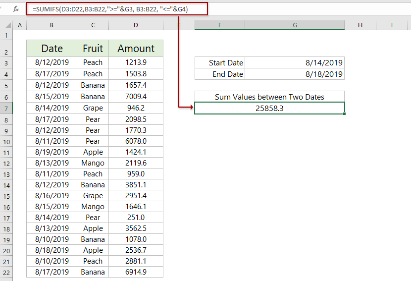
Ko sta na vašem delovnem listu dva seznama, kot je prikazan desni posnetek zaslona, ​​je eden seznam datumov, drugi pa seznam vrednosti. In želite povzeti vrednosti samo med dvema datumoma, na primer, sešteti vrednosti med 3 in 4, kako jih lahko hitro izračunate? Zdaj vam predstavljam formulo za njihovo povzemanje v Excelu.


Vsote vrednosti med dvema datumoma s formulo v Excelu

Na srečo obstaja formula, ki lahko v Excelu sešteje vrednosti med dvema datumoma.

Izberite prazno celico in vnesite spodnjo formulo ter pritisnite Vnesite . In zdaj boste dobili rezultat izračuna. Oglejte si posnetek zaslona:

=SUMIFS(B2:B8,A2:A8,">="&E2,A2:A8,"<="&E3)

Opombe: V zgornji formuli,

  • D3: D22 je seznam vrednosti, ki ga boste povzeli
  • B3: B22 je seznam datumov, na podlagi katerega boste sešteli
  • G3 je celica z začetnim datumom
  • G4 je celica s končnim datumom
note trak Formula je preveč zapletena, da bi si jo zapomnili? Shranite formulo kot vnos samodejnega besedila za nadaljnjo uporabo z enim samim klikom v prihodnosti!
Preberite več ...     Brezplačen preizkus

Preprosto seštevajte podatke v vsakem poslovnem letu, vsakih pol leta ali vsak teden v Excelu

Funkcija posebne časovne razvrstitve vrtilne tabele, ki jo ponuja Kutools za Excel, lahko doda pomožni stolpec za izračun proračunskega leta, pol leta, številke tedna ali dneva v tednu na podlagi določenega stolpca z datumom in omogoča enostavno štetje, vsoto ali povprečni stolpci na podlagi izračunanih rezultatov v novi vrtilni tabeli.


Kutools za Excel - Napolnite Excel z več kot 300 osnovnimi orodji. Uživajte v 30-dnevnem BREZPLAČNEM preskusu s polnimi funkcijami brez kreditne kartice! Get It Now


Vsote vrednosti med dvema datumoma s filtrom v Excelu

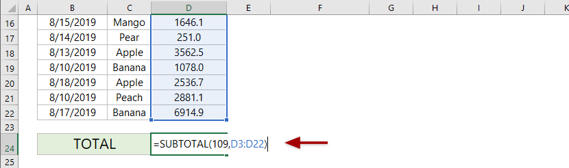
Če morate vrednosti sešteti med dvema datumoma in se časovno obdobje pogosto spreminja, lahko dodate filter za določen obseg in nato uporabite funkcijo SUBTOTAL za seštevanje med določenim časovnim obdobjem v Excelu.

1. Izberite prazno celico, vnesite pod formulo in pritisnite tipko Enter.

= VSEBINA (109, D3: D22)

Opomba: V zgornji formuli 109 pomeni vsoto filtriranih vrednosti, D3: D22 označuje seznam vrednosti, ki ga boste sešteli.

2. Izberite naslov obsega in dodajte filter s klikom datum > filter.

3. V glavi stolpca Datum kliknite ikono filtra in izberite Datumski filtri > Med. V pogovorno okno Samodejni filter po potrebi vnesite začetni in končni datum in kliknite na OK . Skupna vrednost se bo samodejno spremenila glede na filtrirane vrednosti.


Sorodni članki:

Najboljša pisarniška orodja za produktivnost

🤖 Kutools AI Aide: Revolucionirajte analizo podatkov na podlagi: Inteligentna izvedba   |  Ustvari kodo  |  Ustvarite formule po meri  |  Analizirajte podatke in ustvarite grafikone  |  Prikličite funkcije Kutools...
Priljubljene funkcije: Poiščite, označite ali identificirajte dvojnike   |  Izbriši prazne vrstice   |  Združite stolpce ali celice brez izgube podatkov   |   Krog brez formule ...
Super iskanje: Več kriterijev VLookup    Multiple Value VLookup  |   VLookup na več listih   |   Nejasno iskanje ....
Napredni spustni seznam: Hitro ustvarite spustni seznam   |  Odvisni spustni seznam   |  Večkrat izberite spustni seznam ....
Upravitelj stolpcev: Dodajte določeno število stolpcev  |  Premakni stolpce  |  Preklop stanja vidnosti skritih stolpcev  |  Primerjaj obsege in stolpce ...
Predstavljene funkcije: Mrežni fokus   |  Pogled oblikovanja   |   Velika vrstica formule    Upravitelj delovnih zvezkov in listov   |  Knjižnica virov (Samodejno besedilo)   |  Izbirnik datuma   |  Združite delovne liste   |  Šifriranje/dešifriranje celic    Pošljite e-pošto po seznamu   |  Super filter   |   Poseben filter (filter krepko/ležeče/prečrtano ...) ...
15 najboljših kompletov orodij12 Besedilo Orodja (dodajanje besedila, Odstrani znake,...)   |   50 + Graf Vrste (Gantt Chart,...)   |   40+ Praktično Formule (Izračunajte starost glede na rojstni dan,...)   |   19 vstavljanje Orodja (Vstavite kodo QR, Vstavi sliko s poti,...)   |   12 Pretvorba Orodja (Številke v besede, Pretvorba valut,...)   |   7 Spoji in razdeli Orodja (Napredne kombinirane vrstice, Razdeljene celice,...)   |   ... in več

Napolnite svoje Excelove spretnosti s Kutools za Excel in izkusite učinkovitost kot še nikoli prej. Kutools za Excel ponuja več kot 300 naprednih funkcij za povečanje produktivnosti in prihranek časa.  Kliknite tukaj, če želite pridobiti funkcijo, ki jo najbolj potrebujete...

Opis


Kartica Office prinaša vmesnik z zavihki v Office in poenostavi vaše delo

  • Omogočite urejanje in branje z zavihki v Wordu, Excelu, PowerPointu, Publisher, Access, Visio in Project.
  • Odprite in ustvarite več dokumentov v novih zavihkih istega okna in ne v novih oknih.
  • Poveča vašo produktivnost za 50%in vsak dan zmanjša na stotine klikov miške za vas!
Comments (48)
No ratings yet. Be the first to rate!
This comment was minimized by the moderator on the site
INVOICE DATE TOTAL
01-09-2021 19817
02-09-2021 44791
03-09-2021 26780
03-09-2021 58500
03-09-2021 2029

04-09-2021 79260
04-09-2021 2120
04-09-2021 9187
04-09-2021 5698
04-09-2021 1400
04-09-2021 1900
04-09-2021 7500
04-09-2021 830


i have above data in one sheet and i need date wise total value as below in another sheet,01-09-2021 19817
02-09-2021 44791
03-09-2021 87309
04-09-2021 107895

pls give formula details for itsanjay
This comment was minimized by the moderator on the site
Hi Jett,
You can use the SUMIFS function to sum by multiple criteria simultaneously.
=SUMIFS(sum_range, criteria_range1, criteria1, criteria_range2, criteria2,…, criteria_rangeN, criteriaN)
This comment was minimized by the moderator on the site
What if there are multiple columns to sum up like one for interest, one for penalty, and one for principal amount? and it still need to be between two dates
This comment was minimized by the moderator on the site
hi i have a question related to your topic,if the case is like thisDATE AMOUNT17 SEP 70.000 60.00018 SEP 30.00019 SEP 20.000 10.000IF i use sum if between date 17 sept to 19 sept the 60.000 & 10.000 can't be include in the total.what formulas should i use to include the 60.000 and 10.000 in the total?
This comment was minimized by the moderator on the site
Hi, i have a question related to sumifs:

want to calculate a sum between two dates e.g. start of date and end of date, but at times there are payments which were made in a new month but connected to the expense month, For example if a payment date is Oct 5th but the payment is for September and I would like to show this payment for the month of September, the formula should ignore the Oct 5th date and consider the payment in September. How do i do that
This comment was minimized by the moderator on the site
Help! I can only get this formula to work if I convert to a MM/DD/YYYY format but all of my data is DD/MM/YYYY. The cells are formatted correctly but the formula doesn't work unless I change from eg. 14/01/2020 to 01/14/2020.
This comment was minimized by the moderator on the site
Hi,

can you help me to calculate two working experiences in excel.

Ex: 12 Yeas 3 Months 5 Days - CDB Finance company

9 Years 4 Months 7 Days - Commercial Bank

These are two working experiences in two working places of one person. how to sum these two experiences as a total experience in excel. Please help me.
This comment was minimized by the moderator on the site
Hi Ayesha,
We can suppose the start is 1900/1/0, and add the two date periods to get the end date, and then get the difference between the start date and end date as attached image shown.
Two formulas used:
In Cell B7: =DATE(YEAR(0)+B4+B5,MONTH(0)+C4+C5,DAY(0)+D4+D5)
In Cell B9: =DATEDIF(B1,B7,"Y")&" Years, "&DATEDIF(B1,B7,"YM")&" Months, "&DATEDIF(B1,B7,"MD")&" Days"
This comment was minimized by the moderator on the site
Hi all,

What if one would like to make a date range non-mandatory?

Meaning, let's say that I have two cells with dates in them that are used as my beginning and end date threshold, but when those cells aren't populated, the sum for all dates is pulled from the data set.

My formula (below) has two match criteria with the date ranges at the back of the formula. What I'm trying to do is only filter the sum by the date range if a condition is met (ideally a cell that acts as select Yes or No on "Do you want to limit the sum to a specific date range?"

=SUMIFS(BURN_DATA!$S:$S,BURN_DATA!$R:$R,$A12,BURN_DATA!$H:$H,I$3,BURN_DATA!O:O,">="&I9,BURN_DATA!O:O,"<="&J9)


THANKS IN ADVANCE!
This comment was minimized by the moderator on the site
Aloha, I'm trying to figure out how to sum another column of units, when one column of dates is sequential. Example: I have rows with dates, Mar 1, Mar 2, mar3, then marc 6,7, then march 10.
I need to sum the corresponding units in of another column for mar 1-3, mar 6-7 and mar 10.
This comment was minimized by the moderator on the site
Hi David,
You can use methods introduced in this webpage to sum each period one by one.
Or you can add a helper column before the date column as attached image shown, and then apply the Subtotal feature.
This comment was minimized by the moderator on the site
I am trying to create a holiday calendar to calculate the following information:

Start Date:
End Date (if there is one, otherwise calculate on the entire holiday year_
No of Holidays
Holiday year runs from 01/04 to 31/03 with an entitlement of 20 days plus bank holidays

any help is much appreciated
There are no comments posted here yet
Load More
Please leave your comments in English
Posting as Guest
×
Rate this post:
0   Characters
Suggested Locations