Preskoči na glavno vsebino

Kako pretvoriti datum v proračunsko leto / četrtletje / mesec v Excelu?

Če imate na delovnem listu seznam datumov in želite hitro potrditi poslovno leto / četrtletje / mesec teh datumov, lahko preberete to vadnico, mislim, da boste morda našli rešitev.

Pretvori datum v proračunsko leto

Pretvori datum v davčno četrtletje

Pretvori datum v davčni mesec


puščica modri desni mehurček Pretvori datum v proračunsko leto

1. Izberite celico in vanjo vnesite številko fiskalnega leta, ki se začne z mesecem, tukaj se fiskalno leto mojega podjetja začne 1. julija in vtipkam 7. Oglejte si posnetek zaslona:
doc-convert-fiskalno-leto-1

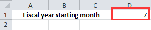
2. Nato lahko vnesete to formulo =YEAR(DATE(YEAR(A4),MONTH(A4)+($D$1-1),1)) v celico poleg vaših datumov, nato povlecite ročico za polnjenje v obseg, ki ga potrebujete.doc-convert-fiskalno-leto-2

Nasvet: V zgornji formuli A4 označuje datumsko celico, D1 pa mesec, v katerem se začne proračunsko leto.


puščica modri desni mehurček Pretvori datum v davčno četrtletje

Če želite datum pretvoriti v davčno četrtletje, lahko storite naslednje:

1. Najprej morate narediti tabelo, kot je prikazano spodaj. V prvo vrstico naštejte vse mesece v letu, nato v drugo vrstico vnesite relativno številko davčnega četrtletja za vsak mesec. Oglejte si posnetek zaslona:
doc-convert-fiskalno-leto-3

2. Nato v celico poleg stolpca z datumom vnesite to formulo = IZBERI (MESEC (A6), 3,3,3,4,4,4,1,1,1,2,2,2) vanj, nato povlecite ročico za polnjenje v obseg, ki ga potrebujete.doc-convert-fiskalno-leto-4

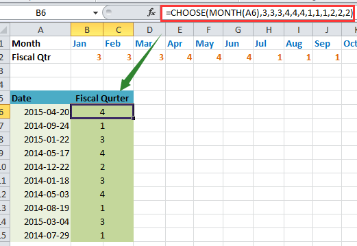
Nasvet: V zgornji formuli je A6 datumska celica, številčna serija 3,3,3… pa fiskalna četrtinska serija, ki ste jo vnesli v 1. koraku.


puščica modri desni mehurček Pretvori datum v davčni mesec

Če želite datum pretvoriti v davčni mesec, morate najprej sestaviti tudi tabelo.

1. V prvo vrstico vnesite vse mesece v letu, nato v drugo vrstico vnesite relativno številko davčnega meseca za vsak mesec. Oglejte si posnetek zaslona:doc-convert-fiskalno-leto-5

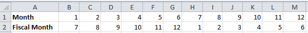
2. Nato v celico poleg stolpca vnesite to formulo = IZBERI (MESEC (A6), 7,8,9,10,11,12,1,2,3,4,5,6) vanj in s to formulo povlecite ročico za polnjenje do želenega obsega. doc-convert-fiskalno-leto-6

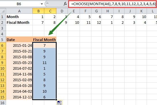
Nasvet: V zgornji formuli je A6 datumska celica, številčna serija 7,8,9… pa številčna številka davčnega meseca, ki jo vnesete v 1. koraku.


Hitro pretvorite nestandardni datum v standardno oblikovanje datuma (mm / dd / llll)

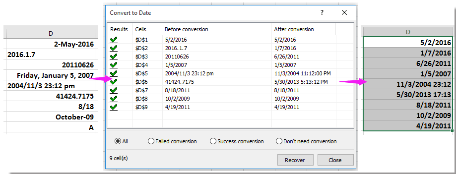
Včasih boste morda prejeli delovne liste z več nestandardnimi datumi in če jih boste pretvorili v standardno obliko zapisa datuma, saj je mm / dd / llll morda za vas težavno. Tukaj Kutools za Excel's Pretvori v datum lahko te nestandardne datume z enim klikom hitro pretvori v standardno oblikovanje datuma.  Kliknite za brezplačno popolno preizkusno različico v 30 dneh!
datum pretvorbe doc
 
Kutools za Excel: z več kot 300 priročnimi dodatki za Excel lahko brezplačno preizkusite brez omejitev v 30 dneh.

Najboljša pisarniška orodja za produktivnost

🤖 Kutools AI Aide: Revolucionirajte analizo podatkov na podlagi: Inteligentna izvedba   |  Ustvari kodo  |  Ustvarite formule po meri  |  Analizirajte podatke in ustvarite grafikone  |  Prikličite funkcije Kutools...
Priljubljene funkcije: Poiščite, označite ali identificirajte dvojnike   |  Izbriši prazne vrstice   |  Združite stolpce ali celice brez izgube podatkov   |   Krog brez formule ...
Super iskanje: Več kriterijev VLookup    Multiple Value VLookup  |   VLookup na več listih   |   Nejasno iskanje ....
Napredni spustni seznam: Hitro ustvarite spustni seznam   |  Odvisni spustni seznam   |  Večkrat izberite spustni seznam ....
Upravitelj stolpcev: Dodajte določeno število stolpcev  |  Premakni stolpce  |  Preklop stanja vidnosti skritih stolpcev  |  Primerjaj obsege in stolpce ...
Predstavljene funkcije: Mrežni fokus   |  Pogled oblikovanja   |   Velika vrstica formule    Upravitelj delovnih zvezkov in listov   |  Knjižnica virov (Samodejno besedilo)   |  Izbirnik datuma   |  Združite delovne liste   |  Šifriranje/dešifriranje celic    Pošljite e-pošto po seznamu   |  Super filter   |   Poseben filter (filter krepko/ležeče/prečrtano ...) ...
15 najboljših kompletov orodij12 Besedilo Orodja (dodajanje besedila, Odstrani znake,...)   |   50 + Graf Vrste (Gantt Chart,...)   |   40+ Praktično Formule (Izračunajte starost glede na rojstni dan,...)   |   19 vstavljanje Orodja (Vstavite kodo QR, Vstavi sliko s poti,...)   |   12 Pretvorba Orodja (Številke v besede, Pretvorba valut,...)   |   7 Spoji in razdeli Orodja (Napredne kombinirane vrstice, Razdeljene celice,...)   |   ... in več

Napolnite svoje Excelove spretnosti s Kutools za Excel in izkusite učinkovitost kot še nikoli prej. Kutools za Excel ponuja več kot 300 naprednih funkcij za povečanje produktivnosti in prihranek časa.  Kliknite tukaj, če želite pridobiti funkcijo, ki jo najbolj potrebujete...

Opis


Kartica Office prinaša vmesnik z zavihki v Office in poenostavi vaše delo

  • Omogočite urejanje in branje z zavihki v Wordu, Excelu, PowerPointu, Publisher, Access, Visio in Project.
  • Odprite in ustvarite več dokumentov v novih zavihkih istega okna in ne v novih oknih.
  • Poveča vašo produktivnost za 50%in vsak dan zmanjša na stotine klikov miške za vas!
Comments (27)
No ratings yet. Be the first to rate!
This comment was minimized by the moderator on the site
How to set If formula is target is month i.e 07.2023 , 08.2022 ...
This comment was minimized by the moderator on the site
For Find in FY Year by month
This comment was minimized by the moderator on the site
Hi, I would like to get an OUTPUT as a Date(10/11/2022) in Colum F, from a Fiscal Year (2023) in column A and Month(11) in Colum D. As my fiscal Year starts from November and Ends in October.

Appreciate your help to find a formula in Excel. Thank
This comment was minimized by the moderator on the site
=IF(MONTH(EOMONTH(B4,0))>3,

YEAR(B4)&"-"&RIGHT(YEAR(B4)+1,2),

YEAR(B4)-1&"-"&RIGHT(YEAR(B4),2))
https://excelforfinance1.blogspot.com/2021/05/excel-formula-to-get-financial-year.html </div>;
This comment was minimized by the moderator on the site
Just check this

=IF(MONTH(I8)>3,"FY"&YEAR(I8)&"-"&YEAR(I8)+1,IF(MONTH(I8)<=3,"FY"&YEAR(I8)-1&"-"&YEAR(I8)))

Assume the target is in I8 cell with a date of 8/23/2011 , the out put will be FY2011-2012

Sathish
This comment was minimized by the moderator on the site
worked well...thank you.
This comment was minimized by the moderator on the site
Just check this
=IF(MONTH(I8)>3,"FY"&YEAR(I8)&"-"&YEAR(I8)+1,IF(MONTH(I8)<=3,"FY"&YEAR(I8)-1&"-"&YEAR(I8)))

Assume the target is in I8 cell with a date of 8/23/2011 , the out put will be <span style="letter-spacing: 0.2px; color: inherit; font-family: inherit; font-style: inherit; font-variant-ligatures: inherit; font-variant-caps: inherit; font-weight: inherit;"> </span>
Sathish
This comment was minimized by the moderator on the site
If anyone is looking for a formula to figure out what fiscal/policy year an payment/event happened, even if that fiscal year/policy doesn't start on the first of the month I came up with this.

=YEAR(A4)+((MONTH(A4)>=MONTH($D$1)+(DAY(A4)<Day($D$1)))-1)

D1 in this has to be a full date 01/06/2019 for example.

Also surely a cheeky Vlookup is a better way of doing the quarter formula

=Vlookup(Month(A6),etc.)
This comment was minimized by the moderator on the site
"=Vlookup(Month(A6),etc.)" It's so simple, yet so elegant... not sure why I didn't think of this but this was a huge find. Thank you!
This comment was minimized by the moderator on the site
I came up with a self contained choose() to calculate the fiscal year that doesn't need to use an external cell as an input.
.
Fiscal Year EndCalculation
="June 30, " & (YEAR(E2) +CHOOSE(MONTH(E2),0,0,0,0,0,0,1,1,1,1,1,1))
. * The first part is just a text string
. * & concatenates the first part to the second part which calculatesthe appropriate year.
. * Year(e2) extracts the year number from the date in column E
. * Choose() looks at the month number from that same date.
. For months Jan through June itretrieves the value 0,
. For months July thru Dec itretrieves value 1.
. The retrieved value is added to theyear extracted to give the appropriate year end
“June 30, 2020”.

This is on the assumption that a company is not likely to be changing it's year end. Doesn't work if the sheet is being used for multiple companies with different year ends ...
This comment was minimized by the moderator on the site
Please correct the fiscal-year formula you give above! It does not work unless the fiscal year begins with month 7. This formula will work just fine:

=YEAR(DATE(YEAR(A4),MONTH(A4)+12-($D$1-1),1))

But it is still way more complex than it needs to be. Use Michael's formula (but correct his typo):

=YEAR(A4)+(MONTH(A4)>=$D$1)
This comment was minimized by the moderator on the site
IF YOU WANT TO FIND FISCAL YEAR IN INDIA....
WRITE EXCEL QUERY AS BELOW


=(YEAR(DATE)+(MONTH(DATE)>=4))-1
This comment was minimized by the moderator on the site
You can use below formulae:


Here Col K2 is our date column which is to be converted in format 20XX-XY (e.g. 2017-18).

=IF(MONTH(K2)<4,TEXT(DATE(YEAR(K2)-1,MONTH(K2),DAY(K2)),"YYYY-")&TEXT(DATE(YEAR(K2),MONTH(K2),DAY(K2)),"YY"),TEXT(DATE(YEAR(K2),MONTH(K2),DAY(K2)),"YYYY-")&TEXT(DATE(YEAR(K2)+1,MONTH(K2),DAY(K2)),"YY"))
This comment was minimized by the moderator on the site
You can also use below formula for the same condition :


=IF(MONTH(K2)<4,YEAR(K2)-1&"-"&TEXT(K2,"YY"),YEAR(K2)&"-"&TEXT(K2,"YY")+1)
This comment was minimized by the moderator on the site
Thank you!!
This comment was minimized by the moderator on the site
What a legend. Thank you!
This comment was minimized by the moderator on the site
thank you
There are no comments posted here yet
Load More
Please leave your comments in English
Posting as Guest
×
Rate this post:
0   Characters
Suggested Locations