Preskoči na glavno vsebino

Kako pogojno oblikovati datume, manjše / večje od današnjih v Excelu?

Datume lahko pogojno oblikujete glede na trenutni datum v Excelu. Na primer, lahko formatirate datume pred današnjim dnem ali pa datume, večje od danes. V tej vadnici vam bomo pokazali, kako lahko s funkcijo DANES v pogojnem oblikovanju podrobno označite roke zapadlosti ali prihodnje datume v Excelu.

Pogojni datumi pred datumom danes ali prihodnji datumi v Excelu


Pogojni datumi pred datumom danes ali prihodnji datumi v Excelu

Recimo, da imate seznam datumov, kot je prikazano spodaj. Za oddajo zapadlih rokov in prihodnjih datumov storite naslednje.

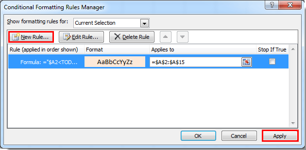
1. Izberite obseg A2: A15 in kliknite Pogojno oblikovanje > Upravljanje pravil pod Domov zavihek. Oglejte si posnetek zaslona:

2. V Ljubljani Upravitelj pravil pogojnega oblikovanja pogovorno okno, kliknite na Novo pravilo gumb.

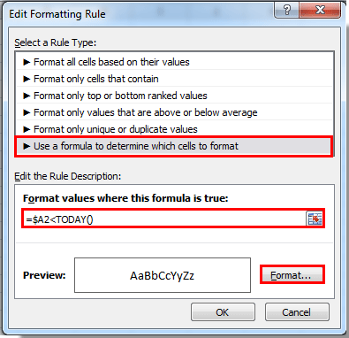
3. V Ljubljani Novo pravilo oblikovanja pogovorno okno, morate:

1). Izberite S formulo določite, katere celice želite formatirati v Izberite vrsto pravila odsek;

2). Za oblikovanje datumov starejših od danes, kopirajte in prilepite formulo = $ A2 v Oblikujte vrednosti, kjer je ta formula resnična škatla;

za oblikovanje prihodnjih datumov, uporabite to formulo = $ A2> DANES ();

3). Kliknite oblikovana . Oglejte si posnetek zaslona:

4. V Ljubljani Oblikuj celice v pogovornem oknu določite obliko datumov zapadlosti ali prihodnjih datumov in kliknite OK gumb.

5. Potem se vrne v Upravitelj pravil pogojnega oblikovanja pogovorno okno. In ustvarjeno je pravilo za oblikovanje rokov. Če želite pravilo uporabiti zdaj, kliknite Uporabi gumb.

6. Če pa želite skupaj uporabiti pravilo zapadlih datumov in pravilo prihodnjih datumov, ustvarite novo pravilo s formulo za oblikovanje prihodnjega datuma, tako da ponovite zgornje korake od 2 do 4.

7. Ko se vrne v Upravitelj pravil pogojnega oblikovanja Ponovno pogovorno okno, vidite, da sta v polju prikazani pravili, kliknite OK za začetek formatiranja.

Nato lahko vidite datume, starejše od danes, in datumi, ki so večji od danes, so uspešno formatirani.

Preprosto pogojno oblikovanje vsake n vrstice v izboru:

Kutools za Excel's Nadomestno zasenčenje vrstic / stolpcev pripomoček vam pomaga enostavno dodati pogojno oblikovanje v vsako n vrstic v Excelovem izboru.
Prenesite celotno 30-dnevno brezplačno pot Kutools za Excel zdaj!


Sorodni članki:

Najboljša pisarniška orodja za produktivnost

🤖 Kutools AI Aide: Revolucionirajte analizo podatkov na podlagi: Inteligentna izvedba   |  Ustvari kodo  |  Ustvarite formule po meri  |  Analizirajte podatke in ustvarite grafikone  |  Prikličite funkcije Kutools...
Priljubljene funkcije: Poiščite, označite ali identificirajte dvojnike   |  Izbriši prazne vrstice   |  Združite stolpce ali celice brez izgube podatkov   |   Krog brez formule ...
Super iskanje: Več kriterijev VLookup    Multiple Value VLookup  |   VLookup na več listih   |   Nejasno iskanje ....
Napredni spustni seznam: Hitro ustvarite spustni seznam   |  Odvisni spustni seznam   |  Večkrat izberite spustni seznam ....
Upravitelj stolpcev: Dodajte določeno število stolpcev  |  Premakni stolpce  |  Preklop stanja vidnosti skritih stolpcev  |  Primerjaj obsege in stolpce ...
Predstavljene funkcije: Mrežni fokus   |  Pogled oblikovanja   |   Velika vrstica formule    Upravitelj delovnih zvezkov in listov   |  Knjižnica virov (Samodejno besedilo)   |  Izbirnik datuma   |  Združite delovne liste   |  Šifriranje/dešifriranje celic    Pošljite e-pošto po seznamu   |  Super filter   |   Poseben filter (filter krepko/ležeče/prečrtano ...) ...
15 najboljših kompletov orodij12 Besedilo Orodja (dodajanje besedila, Odstrani znake,...)   |   50 + Graf Vrste (Gantt Chart,...)   |   40+ Praktično Formule (Izračunajte starost glede na rojstni dan,...)   |   19 vstavljanje Orodja (Vstavite kodo QR, Vstavi sliko s poti,...)   |   12 Pretvorba Orodja (Številke v besede, Pretvorba valut,...)   |   7 Spoji in razdeli Orodja (Napredne kombinirane vrstice, Razdeljene celice,...)   |   ... in več

Napolnite svoje Excelove spretnosti s Kutools za Excel in izkusite učinkovitost kot še nikoli prej. Kutools za Excel ponuja več kot 300 naprednih funkcij za povečanje produktivnosti in prihranek časa.  Kliknite tukaj, če želite pridobiti funkcijo, ki jo najbolj potrebujete...

Opis


Kartica Office prinaša vmesnik z zavihki v Office in poenostavi vaše delo

  • Omogočite urejanje in branje z zavihki v Wordu, Excelu, PowerPointu, Publisher, Access, Visio in Project.
  • Odprite in ustvarite več dokumentov v novih zavihkih istega okna in ne v novih oknih.
  • Poveča vašo produktivnost za 50%in vsak dan zmanjša na stotine klikov miške za vas!
Comments (24)
No ratings yet. Be the first to rate!
This comment was minimized by the moderator on the site
I want to highlight a cell if:
1. today's date is greater than the date in another cell or blank (=TODAY()>'APM Tracker'P14) AND ALSO;
2. If the date in P15 is greater than P14 same highlight color AND ALSO;
3. If the date in P15 is less than P14 I do not want the highlight
This comment was minimized by the moderator on the site
Hey All,

I want to get only past due dates in the particular column. Instead of highlighting the cells with color i need the dates to be picked in the column

Any solution for this....
This comment was minimized by the moderator on the site
Alright, I read through this thread and did not see this question asked/answered. I have a column of future dates. I would like to add conditional formatting to flag that date exactly 30 days before (1st color "Hey you should get this done its due in 30 day's") and 7 days ( 2nd color "You procrastinated and now you have 7 days to complete this"). Any help here?
This comment was minimized by the moderator on the site
Hi Michael,
I am not sure I understand your question clearly. If you want to hight the date which is 30 days and 7 days from today. Please use the following formulas to create two formula rules with different highlighted colors:
=D9=TODAY()+30
=D9=TODAY()+7

https://www.extendoffice.com/images/stories/comments/comment-picture-zxm/conditional-formatting.png
If this is not what you need, please attach a screenshot of your data here.
This comment was minimized by the moderator on the site
To ignore cells that have blanks try this:

=AND($A2<>"",$A2<TODAY())

This assumes the cell you have selected is A2 (change this to whatever cell you have currently selected)
To copy this to the applicable cells, change the "Applies to" to the cell range you need.
This comment was minimized by the moderator on the site
Hi Andy Campbell,
Thank you for sharing.
This comment was minimized by the moderator on the site
Hi
I am trying to use condition formatting to allow a cell to be highlighted when an item is past due based on different turn around times (TAT). I have a column with a submitted date which is then used with the #of days from the TAT to automatically give the due date. Using the following formula, =IF(OR(E3="",A3=""),"",DATE(YEAR(A3),MONTH(A3),DAY(A3)+E3))
The condition formatting currently used is "cell value < today()" applies to +$G:$G.
What I would like to do is use the stop if rule to stop the condition formatting if the date entered in column "H" is < or = to todays date.
Thanks Michelle
This comment was minimized by the moderator on the site
if i want highlight the due date with the conditional : today less or equal 30 days from due date
This comment was minimized by the moderator on the site
I am trying to create conditional formatting that will highlight rows older than 14 days in yellow and highlight rows older than 21 days in red. My date column starts in A2, I have the following rules applied, but only yellow is highlighting and just the date column, not the entire row. Can you help? Scott

1. =ISBLANK(A2)=TRUE
2. =A2<TODAY()-14
3. =A2<TODAY()-21
This comment was minimized by the moderator on the site
I want to ignore blank cells which doesn't have a date i.e I do not want blank cells to be highlighted when I am comparing dates<Today(). Please help
This comment was minimized by the moderator on the site
Hi Madhu,
The first method in this artice can help you solve the problem. Please have a try.
https://www.extendoffice.com/documents/excel/2499-excel-conditional-formatting-ignore-blank-zero.html
This comment was minimized by the moderator on the site
1 colum has the dates in it i want another colum to change colour when this formula is applied.

any ideas?
This comment was minimized by the moderator on the site
Hi grant,
Supposing you want to change the cell color in column B based on dates in column A, please select the column B cells (such as B2:B21), and apply the conditional formatting function with the above formulas =$A2>Today() or =$A2<Today().
This comment was minimized by the moderator on the site
Hello! can anyone help me?

I have =TODAY() formula in A1 and need 3 more rules to work as per below

rule 1 all dates 8 to 14 days older than today

rule 2 : all dates older 14 to 30 days than today

rule 3: all dates 31 or more days older than today
This comment was minimized by the moderator on the site
it should be something like this:

if(*cell*+8>Today();if(*cell*+14<Today();"8-14 from today";"N/A"))
There are no comments posted here yet
Load More
Please leave your comments in English
Posting as Guest
×
Rate this post:
0   Characters
Suggested Locations