Preskoči na glavno vsebino

Kako najti prvi ali zadnji petek vsakega meseca v Excelu?

Običajno je petek zadnji delovni dan v mesecu. Kako lahko poiščete prvi ali zadnji petek glede na določen datum v Excelu? V tem članku vas bomo vodili skozi uporabo dveh formul za iskanje prvega ali zadnjega petka v mesecu.

Poiščite prvi petek v mesecu
Poiščite zadnji petek v mesecu


Poiščite prvi petek v mesecu

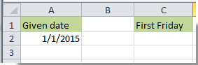
Na primer, v celici A1 je določen datum 1. 2015. 2, kot je prikazano spodaj. Če želite najti prvi petek v mesecu glede na dani datum, storite naslednje.

1. Izberite celico za prikaz rezultata. Tu izberemo celico C2.

2. Kopirajte in prilepite spodnjo formulo, nato pritisnite Vnesite ključ.

=CEILING(EOMONTH(A2,-1)-5,7)+6

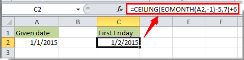
Nato je datum prikazan v celici C2, kar pomeni, da je prvi petek januarja 2015 datum 1/2/2015.

Opombe:

1. Če želite najti prvi petek v drugih mesecih, vnesite določen datum tega meseca v celico A2 in nato uporabite formulo.

2. V formuli je A2 referenčna celica, ki jo določen datum najde. Lahko ga spremenite tako, da ustreza vašim potrebam.

Poiščite zadnji petek v mesecu

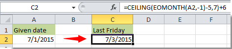
Dani 1. 1. 2015 se nahaja v celici A2, če želite v Excelu poiskati zadnji petek tega meseca, storite naslednje.

1. Izberite celico, v njo kopirajte spodnjo formulo in pritisnite na Vnesite ključ, da dobite rezultat.

=DATE(YEAR(A2),MONTH(A2)+1,0)+MOD(-WEEKDAY(DATE(YEAR(A2),MONTH(A2)+1,0),2)-2,-7)

Nato zadnji petek januarja 2015 prikazuje celico B2.

Opombe: A2 lahko v formuli spremenite v referenčno celico navedenega datuma.


Sorodni članki:

Najboljša pisarniška orodja za produktivnost

🤖 Kutools AI Aide: Revolucionirajte analizo podatkov na podlagi: Inteligentna izvedba   |  Ustvari kodo  |  Ustvarite formule po meri  |  Analizirajte podatke in ustvarite grafikone  |  Prikličite funkcije Kutools...
Priljubljene funkcije: Poiščite, označite ali identificirajte dvojnike   |  Izbriši prazne vrstice   |  Združite stolpce ali celice brez izgube podatkov   |   Krog brez formule ...
Super iskanje: Več kriterijev VLookup    Multiple Value VLookup  |   VLookup na več listih   |   Nejasno iskanje ....
Napredni spustni seznam: Hitro ustvarite spustni seznam   |  Odvisni spustni seznam   |  Večkrat izberite spustni seznam ....
Upravitelj stolpcev: Dodajte določeno število stolpcev  |  Premakni stolpce  |  Preklop stanja vidnosti skritih stolpcev  |  Primerjaj obsege in stolpce ...
Predstavljene funkcije: Mrežni fokus   |  Pogled oblikovanja   |   Velika vrstica formule    Upravitelj delovnih zvezkov in listov   |  Knjižnica virov (Samodejno besedilo)   |  Izbirnik datuma   |  Združite delovne liste   |  Šifriranje/dešifriranje celic    Pošljite e-pošto po seznamu   |  Super filter   |   Poseben filter (filter krepko/ležeče/prečrtano ...) ...
15 najboljših kompletov orodij12 Besedilo Orodja (dodajanje besedila, Odstrani znake,...)   |   50 + Graf Vrste (Gantt Chart,...)   |   40+ Praktično Formule (Izračunajte starost glede na rojstni dan,...)   |   19 vstavljanje Orodja (Vstavite kodo QR, Vstavi sliko s poti,...)   |   12 Pretvorba Orodja (Številke v besede, Pretvorba valut,...)   |   7 Spoji in razdeli Orodja (Napredne kombinirane vrstice, Razdeljene celice,...)   |   ... in več

Napolnite svoje Excelove spretnosti s Kutools za Excel in izkusite učinkovitost kot še nikoli prej. Kutools za Excel ponuja več kot 300 naprednih funkcij za povečanje produktivnosti in prihranek časa.  Kliknite tukaj, če želite pridobiti funkcijo, ki jo najbolj potrebujete...

Opis


Kartica Office prinaša vmesnik z zavihki v Office in poenostavi vaše delo

  • Omogočite urejanje in branje z zavihki v Wordu, Excelu, PowerPointu, Publisher, Access, Visio in Project.
  • Odprite in ustvarite več dokumentov v novih zavihkih istega okna in ne v novih oknih.
  • Poveča vašo produktivnost za 50%in vsak dan zmanjša na stotine klikov miške za vas!
Comments (12)
Rated 5 out of 5 · 1 ratings
This comment was minimized by the moderator on the site
Even shorter 😅
=lambda(Date;WeekDay;EOMONTH(Date;0)-WEEKDAY(EOMONTH(Date;0);WeekDay+10)+1
Where "WeekDay" parameter is 1=Monday, 7=Sunday
This comment was minimized by the moderator on the site
=lambda(Date;WeekDay;EOMONTH(Date;0)-WEEKDAY(EOMONTH(Date;0);WeekDay+10)+1)

I forgot a bracket at the end
This comment was minimized by the moderator on the site
Vậy công thức tính thứ sáu tuần thứ 2 của tháng như thế nào vậy ban?
This comment was minimized by the moderator on the site
Hi Tâm Cao Điền,
Suppose you want to calculate the second friday of the month based on the given date in A1, you can try the following formula:
=A18-DAY(A18)+CHOOSE(WEEKDAY(A18-DAY(A18),2),11,10,9,8,14,13,12)
This comment was minimized by the moderator on the site
porque cuando lo pruebo tal cual me sale error ?
o sea estoy copiando y pegando y no funciona

alguien sabe?
This comment was minimized by the moderator on the site
Hi andre,
Can you tell me which formula you used in the post? And what error your are experiencing?
This comment was minimized by the moderator on the site
Why not make the "last Friday" formula: =CEILING(EOMONTH(A2,0)-5,7)-1? That works for all dates I have tried....
This comment was minimized by the moderator on the site
Hi Eric,
I hop you are still on this forum and receive my reply.
Thanks so much for an EASY formula. I've never encountered =CEILING.
Rated 5 out of 5
This comment was minimized by the moderator on the site
Hi Eric,
Thanks for sharing it.
This comment was minimized by the moderator on the site
Hello and thank you for this formula. I am not an Excel guru and acnnot easily work out how to change this formula for the last Friday to be the Last Monday, or any other day. Can you please explain how to interpret this.
This comment was minimized by the moderator on the site
Matt,

The way the formula works is: First we find the last day of the month with the EOMONTH() function. For the last day of the current month, we use "0" as the month offset. For the previous month, it would be -1. (Either "=EOMONTH(A2,0)" or "=EOMONTH(A2,-1)".)

Then, in the "=CEILING()" function, we subtract the number of days required to bring us back to Sunday from the day for which we are searching. (For Tuesday, it would be -2, so we make the formula so far: "=CEILING(EOMONTH(A2,0)-2...."

We use the "significance" value of "7" because weeks are seven days long (of course).This finds the date of either the previous Saturday, or the following Saturday (Excel dates started with 1/1/1900, which was a Sunday. So if you enter a "1" in cell A2 with the Long Date format, the cell would read: "Sunday, January 1, 1900".). For that reason, the =CEILING() function, using "7" as the "significance" argument returns Saturday, which is always a multiple of 7 in Excel. Now the formula is "=CEILING(EOMONTH(A2,0)-2,7...".

Now we need to return the date to a Tuesday, so we either subtract 4 for the last Tuesday of the month, or add 3 for the first Tuesday of the next month. So the final formula is, respectively, either "=CEILING(EOMONTH(A2,0)-2,7)-4" or "=CEILING(EOMONTH(A2,0)-2,7)+3".

We can work through the math by assuming the last day of the month is either a Monday (assume its value is 9 - for ease of illustration, so the values do not go negative) or a Wednesday (assume value 11). "EOMONTH()" will return either of those days (9 or 11). Subtracting 2 results in the previous Saturday (value 7) or Monday (value 9), respectively. The CEILING() function then returns, respectively, the previous Saturday (value 7, because the ceiling of 7 with significance 7 is 7) or the current Saturday (value 14, because the ceiling of 9, significance 7, is 14). Subtracting 4 results in the previous Tuesday (value 3) or the current week's Tuesday (value 10), respectively. For the first Tuesday of the following month, adding 3 to the Saturday value (7 or 14) returns either Tuesday value 10, or Tuesday value 17, respectively.


Hopefully that helps you understand so that you can modify the formula as necessary. You can even change it to find the second Tuesday, or second to last Tuesday, by adding or subtracting an additional 7, respectively.
This comment was minimized by the moderator on the site
Hi Matt,
You just need to change the last number -7 to -1 to solove the problem.
=DATE(YEAR(A2),MONTH(A2)+1,0)+MOD(-WEEKDAY(DATE(YEAR(A2),MONTH(A2)+1,0),2)-2,-1)
There are no comments posted here yet
Please leave your comments in English
Posting as Guest
×
Rate this post:
0   Characters
Suggested Locations