Preskoči na glavno vsebino

Kako zaokrožiti datum na prejšnji ali naslednji delovni dan v Excelu?

doc-krog-do-prejšnja nedelja-1
Včasih boste morda morali dobiti prejšnji ali naslednji določen dan v tednu, kot je nedelja, na podlagi datuma, kot je prikazan levi posnetek zaslona. Tukaj ta vadnica ponuja dve formuli za enostavno obravnavo tega opravila v Excelu.
Zaokrožen datum na naslednji določen delovni dan
Zaokrožen datum na prejšnji dan v tednu

puščica modri desni mehurček Okrogli datum na naslednji določen delovni dan

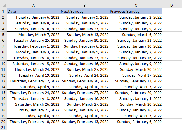
Tukaj na primer, da dobite naslednjo nedeljo datumov v stolpcu A

1. Izberite celico, v katero želite postaviti naslednji nedeljski datum, nato prilepite ali vnesite spodnjo formulo:

=IF(MOD(A2-1,7)>7,A2+7-MOD(A2-1,7)+7,A2+7-MOD(A2-1,7))

2. Nato pritisnite Vnesite tipko, da dobite prvo naslednjo nedeljo, ki je prikazana kot 5-mestna številka, nato povlecite samodejno izpolnjevanje navzdol, da dobite vse rezultate.

doc-krog-do-prejšnja nedelja-1

3. Nato pustite celice formule izbrane in pritisnite Ctrl + 1 tipke za prikaz Oblikuj celice pogovorno okno, nato pod Število jeziček, izberite Datum in izberite eno vrsto datuma na desnem seznamu, kot jo potrebujete. Kliknite OK.

doc-krog-do-prejšnja nedelja-1

Zdaj so rezultati formule prikazani v obliki datuma.

doc-krog-do-prejšnja nedelja-1

Za naslednji dan v tednu uporabite spodnje formule:

Delovni dan Formula
Nedelja =IF(MOD(A2-1,7)>7,A2+7-MOD(A2-1,7)+7,A2+7-MOD(A2-1,7))
Sobota =IF(MOD(A2-1,7)>6,A2+6-MOD(A2-1,7)+7,A2+6-MOD(A2-1,7))
Petek =IF(MOD(A2-1,7)>5,A2+5-MOD(A2-1,7)+7,A2+5-MOD(A2-1,7))
Četrtek =IF(MOD(A2-1,7)>4,A2+4-MOD(A2-1,7)+7,A2+4-MOD(A2-1,7))
Sreda =IF(MOD(A1-1,7)>3,A1+3-MOD(A1-1,7)+7,A1+3-MOD(A1-1,7))
; torek =IF(MOD(A1-1,7)>2,A1+2-MOD(A1-1,7)+7,A1+2-MOD(A1-1,7))
Ponedeljek =IF(MOD(A1-1,7)>1,A1+1-MOD(A1-1,7)+7,A1+1-MOD(A1-1,7))

puščica modri desni mehurček Okrogel datum na prejšnji določen dan v tednu

Tukaj na primer dobite prejšnjo nedeljo datumov v stolpcu A

1. Izberite celico, v katero želite postaviti naslednji nedeljski datum, nato prilepite ali vnesite spodnjo formulo:

=A2-TEDNIK (A2,2)

2. Nato pritisnite Vnesite tipko, da dobite prvo naslednjo nedeljo, nato povlecite samodejno izpolnjevanje navzdol, da dobite vse rezultate.

doc-krog-do-prejšnja nedelja-1

Če želite spremeniti obliko datuma, pustite celice formule izbrane, pritisnite Ctrl + 1 tipke za prikaz Oblikuj celice pogovorno okno, nato pod Število jeziček, izberite Datum in izberite eno vrsto datuma na desnem seznamu, kot jo potrebujete. Kliknite OK.

doc-krog-do-prejšnja nedelja-1

Zdaj so rezultati formule prikazani v obliki datuma.

doc-krog-do-prejšnja nedelja-1

Za pridobitev prejšnjega drugega dne v tednu uporabite spodnje formule:

Delovni dan Formula
Nedelja =A2-TEDNIK (A2,2)
Sobota =IF(WEEKDAY(A2,2)>6,A2-WEEKDAY(A2,1),A2-WEEKDAY(A2,2)-1)
Petek =IF(WEEKDAY(A2,2)>5,A2-WEEKDAY(A2,2)+5,A2-WEEKDAY(A2,2)-2)
Četrtek =IF(WEEKDAY(A2,2)>4,A2-WEEKDAY(A2,2)+4,A2-WEEKDAY(A2,2)-3)
Sreda =IF(WEEKDAY(A2,2)>3,A2-WEEKDAY(A2,2)+3,A2-WEEKDAY(A2,2)-4)
; torek =IF(WEEKDAY(A2,2)>2,A2-WEEKDAY(A2,2)+2,A2-WEEKDAY(A2,2)-5)
Ponedeljek =IF(WEEKDAY(A2,2)>1,A2-WEEKDAY(A2,2)+1,A2-WEEKDAY(A2,2)-6)

Zmogljiv pomočnik za datum in čas

O Pomočnik za datum in čas značilnost Kutools za Excel, podpira enostavno seštevanje/odštevanje datuma in čas, izračunavanje razlike med dvema datumoma in izračun starosti glede na rojstni dan.  Kliknite za brezplačno preskusno različico!
doc-krog-do-prejšnja nedelja-1
 
Kutools za Excel: z več kot 200 priročnimi dodatki za Excel, ki jih lahko brezplačno poskusite brez omejitev.

Najboljša pisarniška orodja za produktivnost

🤖 Kutools AI Aide: Revolucionirajte analizo podatkov na podlagi: Inteligentna izvedba   |  Ustvari kodo  |  Ustvarite formule po meri  |  Analizirajte podatke in ustvarite grafikone  |  Prikličite funkcije Kutools...
Priljubljene funkcije: Poiščite, označite ali identificirajte dvojnike   |  Izbriši prazne vrstice   |  Združite stolpce ali celice brez izgube podatkov   |   Krog brez formule ...
Super iskanje: Več kriterijev VLookup    Multiple Value VLookup  |   VLookup na več listih   |   Nejasno iskanje ....
Napredni spustni seznam: Hitro ustvarite spustni seznam   |  Odvisni spustni seznam   |  Večkrat izberite spustni seznam ....
Upravitelj stolpcev: Dodajte določeno število stolpcev  |  Premakni stolpce  |  Preklop stanja vidnosti skritih stolpcev  |  Primerjaj obsege in stolpce ...
Predstavljene funkcije: Mrežni fokus   |  Pogled oblikovanja   |   Velika vrstica formule    Upravitelj delovnih zvezkov in listov   |  Knjižnica virov (Samodejno besedilo)   |  Izbirnik datuma   |  Združite delovne liste   |  Šifriranje/dešifriranje celic    Pošljite e-pošto po seznamu   |  Super filter   |   Poseben filter (filter krepko/ležeče/prečrtano ...) ...
15 najboljših kompletov orodij12 Besedilo Orodja (dodajanje besedila, Odstrani znake,...)   |   50 + Graf Vrste (Gantt Chart,...)   |   40+ Praktično Formule (Izračunajte starost glede na rojstni dan,...)   |   19 vstavljanje Orodja (Vstavite kodo QR, Vstavi sliko s poti,...)   |   12 Pretvorba Orodja (Številke v besede, Pretvorba valut,...)   |   7 Spoji in razdeli Orodja (Napredne kombinirane vrstice, Razdeljene celice,...)   |   ... in več

Napolnite svoje Excelove spretnosti s Kutools za Excel in izkusite učinkovitost kot še nikoli prej. Kutools za Excel ponuja več kot 300 naprednih funkcij za povečanje produktivnosti in prihranek časa.  Kliknite tukaj, če želite pridobiti funkcijo, ki jo najbolj potrebujete...

Opis


Kartica Office prinaša vmesnik z zavihki v Office in poenostavi vaše delo

  • Omogočite urejanje in branje z zavihki v Wordu, Excelu, PowerPointu, Publisher, Access, Visio in Project.
  • Odprite in ustvarite več dokumentov v novih zavihkih istega okna in ne v novih oknih.
  • Poveča vašo produktivnost za 50%in vsak dan zmanjša na stotine klikov miške za vas!
Comments (16)
No ratings yet. Be the first to rate!
This comment was minimized by the moderator on the site
I have tested this but partially incorrect result was out. Why ?
I wanted to get next Friday.

=IF(A2="","",A2+5-Mod(A2-1,7))

I have entered 11/19/2022
The result was past day 11/18/2022
This comment was minimized by the moderator on the site
Thanks for your reminder, the original formula is not enough rigorous indeed. I have updated the formulas and rewrited the tutorial, hope the new formulas can help you.
This comment was minimized by the moderator on the site
Im trying to work out how to use a date, less an amount of days but ensure when subtracting the days it lands on a weekday not a weekend.
Any formulas??
This comment was minimized by the moderator on the site
Hi Everyone,
I use the formula below to round to the next Thursday where A1 is the cell with your original date and 14 is for Thursday. You can use other numbers for other days if required. 11=Monday, 12=Tuesday, 13=Wednesday, etc...

Also, you can use a 1 instead of an 8 to get the Thursday before your original date in A1. If your original date is already a Thursday the formula will produce the same date as in A1.

I hope this helps!

=A1+(0-WEEKDAY(A1,14)+8)
This comment was minimized by the moderator on the site
Thank you! This worked :)
This comment was minimized by the moderator on the site
I put this into google sheets and to make the dates become next thursday but I have not been able to get it to work especially for the dates right after thursdays. =IF(L2="","",L2+4-MOD(L2-1,4)) is the function i used to make it thursday but not all dates were thursday.
This comment was minimized by the moderator on the site
to clarify, all dates become thursday, but friday and saturday will not convert to the next weeks thursday instead they will go back a day or two to the previous thursday instead going to next weeks thursday, is there any way to fix this in the function =IF(L4="","",L4+4-MOD(L4-1,7))
This comment was minimized by the moderator on the site
Hi Kisho,

I use the formula below to round to the next Thursday where A1 is the cell with your original date and 14 is for Thursday. You can use other numbers for other days if required. 11=Monday, 12=Tuesday, 13=Wednesday, etc...

Also, you can use a 1 instead of an 8 to get the Thursday before your original date in A1. If your original date is already a Thursday the formula will produce the same date as in A1.

I hope this helps!

=A1+(0-WEEKDAY(A1,14)+8)
This comment was minimized by the moderator on the site
Hi Kisho,
I use the formula below to round to the next Thursday where A1 is the cell with your original date and 14 is for Thursday. You can use other numbers for other days if required. 11=Monday, 12=Tuesday, 13=Wednesday, etc...
Also, you can use a 1 instead of an 8 to get the Thursday before your original date in A1. If your original date is already a Thursday the formula will produce the same date as in A1.
I hope this helps!
=A1+(0-WEEKDAY(A1,14)+8)
This comment was minimized by the moderator on the site
I put this into google sheets and to make the dates become next thursday but I have not been able to get it to work especially for the dates right after thursdays. =IF(L2="","",L2+4-MOD(L2-1,4)) is the function i used to make it thursday but not all dates were thursday.
This comment was minimized by the moderator on the site
Si quiero la fecha del próximo viernes cómo debo modificar las variables? Gracias
This comment was minimized by the moderator on the site
Sorry, I cannot understand, could you speak in English?
This comment was minimized by the moderator on the site
hi guys,

I used the formula below, I hope it works for you.
IF(WEEKDAY(H2,16)<>7,(7-WEEKDAY(H2,16))+H2,H2) where H2 is the date that you want to round up to the next day of the week (in my case for Friday) and the 16 is the format to start the date with Saturday as #1 and Friday as #7.
This comment was minimized by the moderator on the site
Your round to previous Sunday is flawed. Even shows as much on your sheet.
This comment was minimized by the moderator on the site
So, what would be the correct formula to first check to see if a cell has a date, else leave it blank and make the date the fall on a Friday before if the date falls on a Saturday or Sunday?
This comment was minimized by the moderator on the site
I found a workaround for to the previous Friday. You can change the switch "results" as needed to round to different days.=H3-SWITCH(TEXT(H3, "DDD"), "Mon", 3, "Tue", 4, "Wed", 5, "Thu", 6, "Fri", 0, "Sat", 1, "Sun", 2)
=[date]-SWITCH(TEXT([date], "DDD"), "Mon", 3, "Tue", 4, "Wed", 5, "Thu", 6, "Fri", 0, "Sat", 1, "Sun", 2)
There are no comments posted here yet
Please leave your comments in English
Posting as Guest
×
Rate this post:
0   Characters
Suggested Locations