Preskoči na glavno vsebino

Kako vlookup najti prvo, drugo ali nto vrednost ujemanja v Excelu?

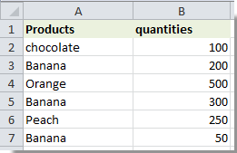
Recimo, da imate dva stolpca z izdelki in količinami, kot je prikazano spodaj. Kaj bi storili, če želite hitro ugotoviti količine prve ali druge banane?

Tu vam lahko funkcija vlookup pomaga pri reševanju te težave. V tem članku vam bomo pokazali, kako vlookup poišče prvo, drugo ali nto vrednost ujemanja s funkcijo Vlookup v Excelu.

Vlookup poišče prvo, drugo ali nto vrednost ujemanja v Excelu s formulo

Preprosto poiščite prvo vrednost ujemanja v Excelu s Kutools za Excel


Vlookup poišče prvo, drugo ali nto vrednost ujemanja v Excelu

Naredite naslednje, da poiščete prvo, drugo ali nto vrednost ujemanja v Excelu.

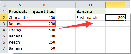
1. V celico D1 vnesite merila, ki jih želite pregledati, tu vnesem Banana.

2. Tu bomo našli prvo ujemajočo se vrednost banane. Izberite prazno celico, na primer E2, kopirajte in prilepite formulo =INDEX($B$2:$B$6,MATCH(TRUE,EXACT($D$1,$A$2:$A$6),0)) v vrstico formule in pritisnite Ctrl + Shift + Vnesite tipke hkrati.

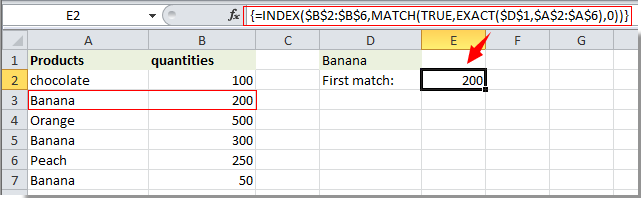
Opombe: V tej formuli je $ B $ 2: $ B $ 6 obseg ustreznih vrednosti; $ A $ 2: $ A $ 6 je obseg z vsemi merili za vlookup; $ D $ 1 je celica, ki vsebuje navedena merila za raziskovanje.

Potem boste dobili prvo ujemanje vrednosti banane v celici E2. S to formulo lahko dobite samo prvo ustrezno vrednost, ki temelji na vaših merilih.

Če želite dobiti katere koli n-je relativne vrednosti, lahko uporabite naslednjo formulo: =INDEX($B$2:$B$6,SMALL(IF($D$1=$A$2:$A$6,ROW($A$2:$A$6)-ROW($A$2)+1),1)) + Ctrl + Shift + Vnesite tipk skupaj, bo ta formula vrnila prvo usklajeno vrednost.

Opombe:

1. Če želite najti drugo vrednost ujemanja, spremenite zgornjo formulo v =INDEX($B$2:$B$6,SMALL(IF($D$1=$A$2:$A$6,ROW($A$2:$A$6)-ROW($A$2)+1),2)), nato pritisnite Ctrl + Shift + Vnesite tipke hkrati. Oglejte si posnetek zaslona:

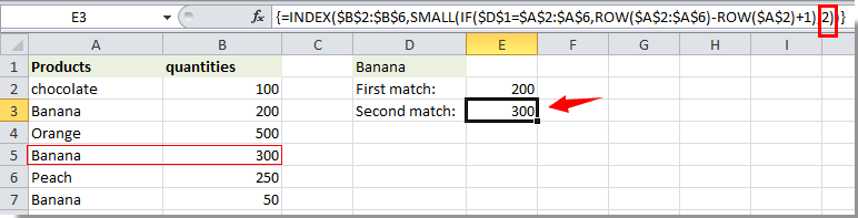
2. Zadnja številka v zgornji formuli pomeni n-to vrednost ujemanja meril vlookup. Če ga spremenite na 3, bo dobil tretjo vrednost ujemanja in se spremeni v n, ugotovila bo n-to vrednost ujemanja.


Vlookup poišče prvo vrednost ujemanja v Excelu z Kutools za Excel

Ylahko preprosto najdete prvo vrednost ujemanja v Excelu, ne da bi si zapomnili formule z Poiščite vrednost na seznamu formula formula za Kutools za Excel.

Pred vložitvijo vloge Kutools za ExcelProsim najprej ga prenesite in namestite.

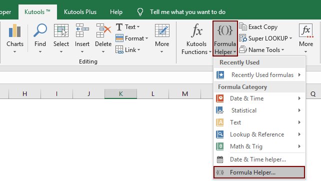
1. Izberite celico za iskanje prve ujemajoče se vrednosti (pravi celica E2) in kliknite Kutools > Pomočnik za formulo > Pomočnik za formulo. Oglejte si posnetek zaslona:

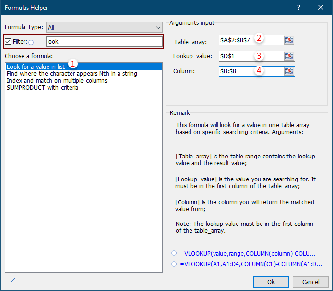
3. V Ljubljani Pomočnik za formulo pogovorno okno, nastavite na naslednji način:

  • 3.1 V Izberite formulo poiščite in izberite Poiščite vrednost na seznamu;
    nasveti: Lahko preverite filter v polje za besedilo vnesite določeno besedo, da hitro filtrirate formulo.
  • 3.2 V Tabela_ matrika izberite polje tabela, ki vsebuje prve vrednosti vrednosti, ki se ujemajo.;
  • 3.2 V Iskalna_vrednost izberite celico, ki vsebuje Merila vrnili boste prvo vrednost na podlagi;
  • 3.3 V Stolpec v stolpcu določite stolpec, iz katerega boste vrnili ujemajočo se vrednost. Ali pa lahko v polje za besedilo vnesete številko stolpca neposredno, kot jo potrebujete.
  • 3.4 Kliknite na OK . Oglejte si posnetek zaslona:

Zdaj bo ustrezna vrednost celice samodejno vnesena v celico C10 na podlagi izbire spustnega seznama.

  Če želite imeti brezplačno (30-dnevno) preskusno različico tega pripomočka, kliknite, če ga želite prenestiin nato nadaljujte z uporabo postopka v skladu z zgornjimi koraki.

Najboljša pisarniška orodja za produktivnost

🤖 Kutools AI Aide: Revolucionirajte analizo podatkov na podlagi: Inteligentna izvedba   |  Ustvari kodo  |  Ustvarite formule po meri  |  Analizirajte podatke in ustvarite grafikone  |  Prikličite funkcije Kutools...
Priljubljene funkcije: Poiščite, označite ali identificirajte dvojnike   |  Izbriši prazne vrstice   |  Združite stolpce ali celice brez izgube podatkov   |   Krog brez formule ...
Super iskanje: Več kriterijev VLookup    Multiple Value VLookup  |   VLookup na več listih   |   Nejasno iskanje ....
Napredni spustni seznam: Hitro ustvarite spustni seznam   |  Odvisni spustni seznam   |  Večkrat izberite spustni seznam ....
Upravitelj stolpcev: Dodajte določeno število stolpcev  |  Premakni stolpce  |  Preklop stanja vidnosti skritih stolpcev  |  Primerjaj obsege in stolpce ...
Predstavljene funkcije: Mrežni fokus   |  Pogled oblikovanja   |   Velika vrstica formule    Upravitelj delovnih zvezkov in listov   |  Knjižnica virov (Samodejno besedilo)   |  Izbirnik datuma   |  Združite delovne liste   |  Šifriranje/dešifriranje celic    Pošljite e-pošto po seznamu   |  Super filter   |   Poseben filter (filter krepko/ležeče/prečrtano ...) ...
15 najboljših kompletov orodij12 Besedilo Orodja (dodajanje besedila, Odstrani znake,...)   |   50 + Graf Vrste (Gantt Chart,...)   |   40+ Praktično Formule (Izračunajte starost glede na rojstni dan,...)   |   19 vstavljanje Orodja (Vstavite kodo QR, Vstavi sliko s poti,...)   |   12 Pretvorba Orodja (Številke v besede, Pretvorba valut,...)   |   7 Spoji in razdeli Orodja (Napredne kombinirane vrstice, Razdeljene celice,...)   |   ... in več

Napolnite svoje Excelove spretnosti s Kutools za Excel in izkusite učinkovitost kot še nikoli prej. Kutools za Excel ponuja več kot 300 naprednih funkcij za povečanje produktivnosti in prihranek časa.  Kliknite tukaj, če želite pridobiti funkcijo, ki jo najbolj potrebujete...

Opis


Kartica Office prinaša vmesnik z zavihki v Office in poenostavi vaše delo

  • Omogočite urejanje in branje z zavihki v Wordu, Excelu, PowerPointu, Publisher, Access, Visio in Project.
  • Odprite in ustvarite več dokumentov v novih zavihkih istega okna in ne v novih oknih.
  • Poveča vašo produktivnost za 50%in vsak dan zmanjša na stotine klikov miške za vas!
Comments (43)
No ratings yet. Be the first to rate!
This comment was minimized by the moderator on the site
You only return first match with VLOOKUP so your article "How To Vlookup Find The First, 2nd Or Nth Match Value In Excel?" does not make any sense....
This comment was minimized by the moderator on the site
Hi Sima,
"VLOOKUP" is a Google search term, so I used it as a keyword for the article title. The main operation of this article is to lookup values. I'm sorry for the misunderstanding.
This comment was minimized by the moderator on the site
What if the next record on col b is a duplicate how do ignore duplicate? Let's Banana has quantities of 200 twice? Can you please help me figure out how to ignore the duplicate?
This comment was minimized by the moderator on the site
Cna anybody Explain the small function with the IF statement for me please? I don't really understand how that array works :(
This comment was minimized by the moderator on the site
The following formulas works perfect for me:
(a) or(b) =IF(H8='Raw Data'!B4,INDEX('Raw Data'!H6:H20,SMALL(IF(C18='Raw Data'!B6:B20,ROW('Raw Data'!B6:B20)-ROW('Raw Data'!B6:B20)+1),1)))

However, I have encountered a problem where there are 7 sets of the same criteria but in different columns:(1) can the above formula (a) be repeated and search in a different cells in a single formula and(2) the above formula (b) only allows up to two sets of the similar search with matched value result but when trying for the third set in the formula as showed below, Microsoft Excel appeared as "You've entered too many arguments for this function."
=<span style="letter-spacing: 0.2px; color: inherit; font-family: inherit; font-style: inherit; font-variant-ligatures: inherit; font-variant-caps: inherit; font-weight: inherit;">IF(H8='Raw Data'!J4,INDEX('Raw Data'!P6:P20,SMALL(IF(C18='Raw Data'!J6:J20,ROW('Raw Data'!J6:J20)-ROW('Raw Data'!J6:J20)+1),1))),</span>
This comment was minimized by the moderator on the site
What do Ctrl + Shift + Enter do?? At the beginning I didn'
This comment was minimized by the moderator on the site
Hi,An array formula needs to hit the Ctrl + Shift + Enter keys simultaneously to get the correct result.
This comment was minimized by the moderator on the site
I have a scenario... How do I get last price of anything for reference... Example: Banana first price was 200... While purchasing for second time; I need to display 200 in my expected price cell and then if I buy that on the day at 220, I will put this value manually as 220... Whenever next time I will buy banana; I need to display 220 from the last purchase price
This comment was minimized by the moderator on the site
Try =INDEX($B$2:$B$6,XMATCH(TRUE,EXACT($D$1,$A$2:$A$6),0,-1))

This is essentially reversing the search order and returning the first match using the XMATCH function.

Better late than never, hopefully helps someone :)
This comment was minimized by the moderator on the site
Perfect explanation, thanks.
This comment was minimized by the moderator on the site
If the first or any of the other entry's for 'banana' column B was blank cell, of which I don't require this number, what changes are required to this formula to skip blank cell in column B.
This comment was minimized by the moderator on the site
Sorry I am using this formula
=INDEX($B$2:$B$6,SMALL(IF($D$1=$A$2:$A$6,ROW($A$2:$A$6)-ROW($A$2)+1),1))
This comment was minimized by the moderator on the site
SOLVED:
=SMALL(IF(A2:A7=D1,IF(B2:B7<>"",B2:B7)),1)

If 2nd or 3rd number required exchange ),1) to 2 or 3

This formula does not require index, as it directly looks at the value in Cell
This comment was minimized by the moderator on the site
Correction to previous formula:
The value was reading either the lesser or greater.

Updated formula
=INDEX($B$2:$B$7,SMALL(IF($A2:$A6=$D$1,IF($B$2:$B$7<>"",ROW($A2:$A6)-ROW($A2)+1)),1))

This skips blank cell and places value of non blank cell. Replace +1 with +2 or +3 for 2nd or 3rd value
This comment was minimized by the moderator on the site
And if you want the last, second last, nth last just add a counter (count the number of events already hapenned) to the end and subtract it by 0,1,n respectively.

Thank you so much! I was searching for this for a long time
This comment was minimized by the moderator on the site
Good Day,
Sorry can't help you with this yet. Thank you for your comment.
This comment was minimized by the moderator on the site
Is it possible to find an average of the non-unique data. Or would it be possible to have a list dropdown on the cell of the various values?
This comment was minimized by the moderator on the site
Good Day,
Sorry can't help you with this yet. Thank you for your comment.
There are no comments posted here yet
Load More
Please leave your comments in English
Posting as Guest
×
Rate this post:
0   Characters
Suggested Locations