Preskoči na glavno vsebino

Kako izvleči edinstvene vrednosti na podlagi meril v Excelu?

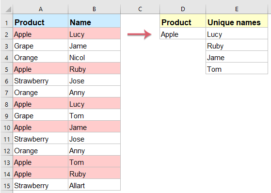
Recimo, da imate levi obseg podatkov, za katerega želite navesti samo enolična imena stolpca B na podlagi določenega merila stolpca A, da dobite rezultat, kot je prikazano spodaj. Kako bi se lahko hitro in enostavno spopadli s to nalogo v Excelu?

Izvlecite edinstvene vrednosti na podlagi meril s formulo matrike

Izvlecite edinstvene vrednosti na podlagi več meril s formulo matrike

Izvlecite edinstvene vrednosti s seznama celic s koristno funkcijo


Izvlecite edinstvene vrednosti na podlagi meril s formulo matrike

Če želite rešiti to nalogo, lahko uporabite kompleksno formulo matrike, naredite naslednje:

1. Vnesite spodnjo formulo v prazno celico, kjer želite navesti rezultat ekstrakcije, v tem primeru jo bom postavil v celico E2 in nato pritisnil Shift + Ctrl + Enter tipke, da dobite prvo unikatno vrednost.

=IFERROR(INDEX($B$2:$B$15, MATCH(0, IF($D$2=$A$2:$A$15, COUNTIF($E$1:$E1, $B$2:$B$15), ""), 0)),"")

2. Nato povlecite ročico za polnjenje navzdol do celic, dokler se ne prikažejo prazne celice, in zdaj so navedene vse edinstvene vrednosti na podlagi določenega merila, glejte posnetek zaslona:

Opomba: V zgornji formuli: B2: B15 obseg stolpcev vsebuje edinstvene vrednosti, iz katerih želite izvleči, A2: A15 je stolpec vsebuje merilo, na katerem temeljiš, D2 označuje merilo, na podlagi katerega želite navesti unikatne vrednosti, in E1 je celica nad vneseno formulo.

Izvlecite edinstvene vrednosti na podlagi več meril s formulo matrike

Če želite izvleči edinstvene vrednosti na podlagi dveh pogojev, je tu še ena formula matrike, ki vam lahko stori uslugo, storite tako:

1. Vnesite spodnjo formulo v prazno celico, kjer želite navesti edinstvene vrednosti, v tem primeru jo bom postavil v celico G2 in nato pritisnil Shift + Ctrl + Enter tipke, da dobite prvo unikatno vrednost.

=IFERROR(INDEX($C$2:$C$15,MATCH(0,COUNTIF(G1:$G$1,$C$2:$C$15)+IF($A$2:$A$15<>$E$2,1,0)+IF($B$2:$B$15<>$F$2,1,0),0)),"")

2. Nato povlecite ročico za polnjenje navzdol do celic, dokler se ne prikažejo prazne celice, in zdaj so navedene vse edinstvene vrednosti, ki temeljijo na določenih dveh pogojih, glejte sliko zaslona:

Opomba: V zgornji formuli: C2: C15 obseg stolpcev vsebuje edinstvene vrednosti, iz katerih želite izvleči, A2: A15 in E2 so prvo območje z merili, na podlagi katerih želite pridobiti edinstvene vrednosti, B2: B15 in F2 so drugo območje z merili, na podlagi katerih želite izvleči edinstvene vrednosti, in G1 je celica nad vneseno formulo.

Izvlecite edinstvene vrednosti s seznama celic s koristno funkcijo

Včasih želite samo izvleči edinstvene vrednosti s seznama celic, tukaj bom priporočil koristno orodje -Kutools za Excel, Z njegovim Izvleči celice z edinstvenimi vrednostmi (vključi prvi dvojnik) pripomoček, lahko hitro izvlečete edinstvene vrednosti.

Opomba:Če želite uporabiti to Izvleči celice z edinstvenimi vrednostmi (vključi prvi dvojnik), najprej bi morali prenesti Kutools za Excelin nato funkcijo hitro in enostavno uporabite.

Po namestitvi Kutools za Excel, naredite tako:

1. Kliknite celico, v katero želite izpisati rezultat. (Opombe: Ne kliknite celice v prvi vrstici.)

2. Nato kliknite Kutools > Pomočnik za formulo > Pomočnik za formulo, glej posnetek zaslona:

3. v Pomočnik za formule pogovorno okno, naredite naslednje:

  • Izberite Besedilo možnost iz Formula tip spustni seznam;
  • Potem izberite Izvleči celice z edinstvenimi vrednostmi (vključi prvi dvojnik) Iz Izberite fromula polje s seznamom;
  • Na desni Vnos argumentov v razdelku izberite seznam celic, za katere želite izvleči edinstvene vrednosti.

4. Nato kliknite Ok gumb, se prvi rezultat prikaže v celici, nato izberite celico in povlecite ročico za polnjenje do celic, v katere želite našteti vse edinstvene vrednosti, dokler niso prikazane prazne celice, glejte sliko zaslona:

Brezplačno prenesite Kutools za Excel zdaj!


Več relativnih člankov:

  • Štejte na seznamu število edinstvenih in ločenih vrednot
  • Recimo, da imate dolg seznam vrednosti z nekaj podvojenimi elementi, zdaj želite prešteti število unikatnih vrednosti (vrednosti, ki so na seznamu samo enkrat) ali ločenih vrednosti (vse različne vrednosti na seznamu pomenijo unikatne vrednosti + 1. podvojene vrednosti) v stolpcu, kot je prikazano na levi sliki zaslona. V tem članku bom govoril o tem, kako ravnati s tem delom v Excelu.
  • Vsota edinstvenih vrednosti na podlagi meril v Excelu
  • Na primer, zdaj imam nabor podatkov, ki vsebujejo stolpca Ime in Naročilo, da v stolpcu Naročilo seštejem samo enolične vrednosti na podlagi stolpca Ime, kot je prikazano na sliki spodaj. Kako hitro in enostavno rešiti to nalogo v Excelu?
  • Združi edinstvene vrednosti v Excelu
  • Če imam dolg seznam vrednosti, ki je zapolnjen z nekaj podvojenimi podatki, želim zdaj najti samo edinstvene vrednosti in jih nato združiti v eno celico. Kako sem se lahko hitro in enostavno spopadel s to težavo v Excelu?

Najboljša pisarniška orodja za produktivnost

🤖 Kutools AI Aide: Revolucionirajte analizo podatkov na podlagi: Inteligentna izvedba   |  Ustvari kodo  |  Ustvarite formule po meri  |  Analizirajte podatke in ustvarite grafikone  |  Prikličite funkcije Kutools...
Priljubljene funkcije: Poiščite, označite ali identificirajte dvojnike   |  Izbriši prazne vrstice   |  Združite stolpce ali celice brez izgube podatkov   |   Krog brez formule ...
Super iskanje: Več kriterijev VLookup    Multiple Value VLookup  |   VLookup na več listih   |   Nejasno iskanje ....
Napredni spustni seznam: Hitro ustvarite spustni seznam   |  Odvisni spustni seznam   |  Večkrat izberite spustni seznam ....
Upravitelj stolpcev: Dodajte določeno število stolpcev  |  Premakni stolpce  |  Preklop stanja vidnosti skritih stolpcev  |  Primerjaj obsege in stolpce ...
Predstavljene funkcije: Mrežni fokus   |  Pogled oblikovanja   |   Velika vrstica formule    Upravitelj delovnih zvezkov in listov   |  Knjižnica virov (Samodejno besedilo)   |  Izbirnik datuma   |  Združite delovne liste   |  Šifriranje/dešifriranje celic    Pošljite e-pošto po seznamu   |  Super filter   |   Poseben filter (filter krepko/ležeče/prečrtano ...) ...
15 najboljših kompletov orodij12 Besedilo Orodja (dodajanje besedila, Odstrani znake,...)   |   50 + Graf Vrste (Gantt Chart,...)   |   40+ Praktično Formule (Izračunajte starost glede na rojstni dan,...)   |   19 vstavljanje Orodja (Vstavite kodo QR, Vstavi sliko s poti,...)   |   12 Pretvorba Orodja (Številke v besede, Pretvorba valut,...)   |   7 Spoji in razdeli Orodja (Napredne kombinirane vrstice, Razdeljene celice,...)   |   ... in več

Napolnite svoje Excelove spretnosti s Kutools za Excel in izkusite učinkovitost kot še nikoli prej. Kutools za Excel ponuja več kot 300 naprednih funkcij za povečanje produktivnosti in prihranek časa.  Kliknite tukaj, če želite pridobiti funkcijo, ki jo najbolj potrebujete...

Opis


Kartica Office prinaša vmesnik z zavihki v Office in poenostavi vaše delo

  • Omogočite urejanje in branje z zavihki v Wordu, Excelu, PowerPointu, Publisher, Access, Visio in Project.
  • Odprite in ustvarite več dokumentov v novih zavihkih istega okna in ne v novih oknih.
  • Poveča vašo produktivnost za 50%in vsak dan zmanjša na stotine klikov miške za vas!
Comments (40)
No ratings yet. Be the first to rate!
This comment was minimized by the moderator on the site
Thank you so much. This was very very helpful. You Rock!!
This comment was minimized by the moderator on the site
hi everyone..
i have problem..
i got blank result even i press ctrl shift enter together..
This comment was minimized by the moderator on the site
Hi all, Can some help me to get all unique values on one single cell
This comment was minimized by the moderator on the site
Hi, this worked well! Although it takes Excel sooooo long to calculate. Just dragging down 15 cells in a column takes about 15min to calculate... if not longer. Is this normal? If this becomes dynamic it will take a hell of alot of computing time.
This comment was minimized by the moderator on the site
Hello. This is really helpful, however, what If I want a formula that lists the unique values based on multiple criteria. eg. I have a data set which has the following data in a table (after each hyphen is a new column but same row):

Company A - £200 - £100
Company A - £300 - £200
Company B - £300 - £200
Company C - £600 - £200
Company B - £100 - £300
Company D - £0 - £600
Company A - £700 - £100

I want a new data table in a new tab which groups the duplicate values without using an array formula. currently I'm grouping using a pivot table and pasting to my new data table. It's a long process but array formulas make my spreadsheet really slow.

Company A - £1200 - £400
Company B - £400 - £500
Company C - £600 - £200
Company D - £0 - £600

Thanks,
K
This comment was minimized by the moderator on the site
Hello, K,
For solving your problem, I can recommend our useful tool- Kutools for Excel, with its Advanced Combine Rows feature, you can deal with this job quickly. Firstly, you should copy and paste your data into a new worksheet, and then apply htis feature as below screenhsot shown.
You can know more about this feature from: https://www.extendoffice.com/product/kutools-for-excel/excel-combine-duplicate-rows.html
Please download Kutools for Excel and install it, then apply this feature. Full feature free trial 30-day, please try.
This comment was minimized by the moderator on the site
Hi! the formula works really well. I would like to add another criterion, i mean, get the unique answers but using two criteria
This comment was minimized by the moderator on the site
Hi, Giancarlo,
to extract unique values based on multiple criteria, any of the below formula can help you: (after pasting the formula, please press Ctrl + Shift + Enter keys together.)
=IFERROR(INDEX($C$2:$C$11, MATCH(0, COUNTIF(G1:$G$1, $C$2:$C$11)+IF($A$2:$A$11<>$E$2, 1, 0)+IF($B$2:$B$11<>$F$2, 1, 0), 0)), "")
=INDEX($C$2:$C$11, MATCH(0, IF(($A$2:$A$11=$E$2)*($B$2:$B$11=$F$2), COUNTIF($G$1:$G1, $C$2:$C$11), ""), 0))
Please try, hope it can help you!
This comment was minimized by the moderator on the site
Hi. I am using the two conditions formula =IFERROR(INDEX($C$2:$C$11, MATCH(0, COUNTIF(G1:$G$1, $C$2:$C$11)+IF($A$2:$A$11<>$E$2, 1, 0)+IF($B$2:$B$11<>$F$2, 1, 0), 0)), "") to extract a unique list and it works great, but I am struggle to add the SMALL function to get the list sorted as well in ascending order. Are you able to help?
This comment was minimized by the moderator on the site
Is there a way to make this work while ALLOWING for duplicate values? For instance, I want all instances of Lucy to be listed in the results.
This comment was minimized by the moderator on the site
Hello, Konstantin,
To extract all corresponding values including the duplicates based on a specific cell criteria, the following array formula can help you, see screenshot:
=IF(ISERROR(INDEX($A$1:$B$17,SMALL(IF($A$1:$A$17=$D$2,ROW($A$1:$A$17)),ROW(1:1)),2)),"",
INDEX($A$1:$B$17,SMALL(IF($A$1:$A$17=$D$2,ROW($A$1:$A$17)),ROW(1:1)),2))

After inserting the formula, please press Shift + Ctrl + Enter keys together to get the correct result, and then drag the fill handle down to get all values.
Hope this can help you, thank you!
This comment was minimized by the moderator on the site
This has worked great for me with a specific lookup value. However, if I wanted to use a wildcard to look up partial values, how would I do that? For example, if I wanted to lookup all the names associated with KT?

I am using this function to look up cells that contain multiple text. For example if each product also had a sub-product within the same cell but I was only looking for names associated with the sub-product "elf".

KTE - elf
KTE- ball
KTE - piano
KTO - elf
KTO- ball
KTO - piano
This comment was minimized by the moderator on the site
For me the formula does not work. I press ctrl shift enter and i still get an error N/A. I would like to add that i prpared exaclty the same data as in tutorial. What is the reason it does not work?
This comment was minimized by the moderator on the site
How would I get this formula to return each of the duplicates instead of one of each of the names? For instance, in the example above, how would I get the results column (B:B) to return Lucy, Ruby, Anny, Jose, Lucy, Anny, Tom? I'm using this as a budget tool pulling to specific account summaries from a general ledger. However, several of the amounts and transaction descriptions are duplicates in the general ledger. Once the first of the duplicated values is pulled, no more of them get pulled.
This comment was minimized by the moderator on the site
Hi, Joe,
To extract all corresponding values based on a specific cell criteria, the following array formula can help you, see screenshot:
=IF(ISERROR(INDEX($A$1:$B$17,SMALL(IF($A$1:$A$17=$D$2,ROW($A$1:$A$17)),ROW(1:1)),2)),"",
INDEX($A$1:$B$17,SMALL(IF($A$1:$A$17=$D$2,ROW($A$1:$A$17)),ROW(1:1)),2))

After inserting the formula, please press Shift + Ctrl + Enter keys together to get the correct result, and then drag the fill handle down to get all values.
Hope this can help you, thank you!
This comment was minimized by the moderator on the site
Last Question: If I want the results column to return all values not associated with KTE or KTO (so, D:D would be Tom, Nocol, Lily, Angelina, Genna), how would I do that?
This comment was minimized by the moderator on the site
Ok, so it works in the master workbook. There is one exception that I haven't been able to determine the cause of: If the array (in my case, the general ledger that I had beginning in row 3) does not begin in Row 1, the returned values are incorrect. What causes this problem, and which term in the formula fixes it? Thanks again for your help with this!
This comment was minimized by the moderator on the site
So far so good. I'm able to duplicate the results in the test sheet, make changes to the array, and then correct the formula to account for the changes I've made. I plan to move this into the master sheet today and see how it works. Thanks for the help!
There are no comments posted here yet
Load More
Please leave your comments in English
Posting as Guest
×
Rate this post:
0   Characters
Suggested Locations