Preskoči na glavno vsebino

Kako zakleniti določene celice, ne da bi v Excelu zaščitili celoten delovni list?

Običajno morate pred urejanjem zaščititi celoten delovni list za zaklepanje celic. Ali obstaja kakšen način zaklepanja celic, ne da bi zaščitili celoten delovni list? Ta članek vam priporoča metodo VBA.

Zaklepanje določenih celic, ne da bi zaščitili celoten delovni list z VBA


Zaklepanje določenih celic, ne da bi zaščitili celoten delovni list z VBA

Če morate zakleniti celici A3 in A5 na trenutnem delovnem listu, vam bo naslednja koda VBA pomagala doseči to, ne da bi zaščitila celoten delovni list.

1. Z desno miškino tipko kliknite jeziček lista in izberite Ogled kode v meniju z desnim klikom.

2. Nato kopirajte in prilepite spodnjo kodo VBA v okno Code. Oglejte si posnetek zaslona:

Koda VBA: zaklepanje določenih celic, ne da bi zaščitili celoten delovni list

Private Sub Worksheet_SelectionChange(ByVal Target As Range)
    If Target.Column = 1 Then
        If Target.Row = 3 Or Target.Row = 5 Then
            Beep
            Cells(Target.Row, Target.Column).Offset(0, 1).Select
        End If
    End If
End Sub

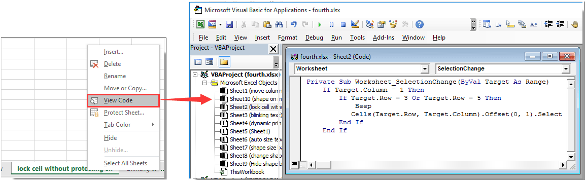
Opombe: V kodi, Stolpec 1, Vrstica = 3 in Vrstica = 5 označite, da se celici A3 in A5 na trenutnem delovnem listu po zagonu kode zakleneta. Lahko jih spremenite po potrebi.

3. Pritisnite druga + Q tipke hkrati, da zaprete tipko Microsoft Visual Basic za aplikacije okno.

Zdaj sta celici A3 in A5 zaklenjeni v trenutnem delovnem listu. Če poskušate na trenutnem delovnem listu izbrati celico A3 ali A5, se kurzor samodejno premakne v desno sosednjo celico.


Sorodni članki:

Najboljša pisarniška orodja za produktivnost

🤖 Kutools AI Aide: Revolucionirajte analizo podatkov na podlagi: Inteligentna izvedba   |  Ustvari kodo  |  Ustvarite formule po meri  |  Analizirajte podatke in ustvarite grafikone  |  Prikličite funkcije Kutools...
Priljubljene funkcije: Poiščite, označite ali identificirajte dvojnike   |  Izbriši prazne vrstice   |  Združite stolpce ali celice brez izgube podatkov   |   Krog brez formule ...
Super iskanje: Več kriterijev VLookup    Multiple Value VLookup  |   VLookup na več listih   |   Nejasno iskanje ....
Napredni spustni seznam: Hitro ustvarite spustni seznam   |  Odvisni spustni seznam   |  Večkrat izberite spustni seznam ....
Upravitelj stolpcev: Dodajte določeno število stolpcev  |  Premakni stolpce  |  Preklop stanja vidnosti skritih stolpcev  |  Primerjaj obsege in stolpce ...
Predstavljene funkcije: Mrežni fokus   |  Pogled oblikovanja   |   Velika vrstica formule    Upravitelj delovnih zvezkov in listov   |  Knjižnica virov (Samodejno besedilo)   |  Izbirnik datuma   |  Združite delovne liste   |  Šifriranje/dešifriranje celic    Pošljite e-pošto po seznamu   |  Super filter   |   Poseben filter (filter krepko/ležeče/prečrtano ...) ...
15 najboljših kompletov orodij12 Besedilo Orodja (dodajanje besedila, Odstrani znake,...)   |   50 + Graf Vrste (Gantt Chart,...)   |   40+ Praktično Formule (Izračunajte starost glede na rojstni dan,...)   |   19 vstavljanje Orodja (Vstavite kodo QR, Vstavi sliko s poti,...)   |   12 Pretvorba Orodja (Številke v besede, Pretvorba valut,...)   |   7 Spoji in razdeli Orodja (Napredne kombinirane vrstice, Razdeljene celice,...)   |   ... in več

Napolnite svoje Excelove spretnosti s Kutools za Excel in izkusite učinkovitost kot še nikoli prej. Kutools za Excel ponuja več kot 300 naprednih funkcij za povečanje produktivnosti in prihranek časa.  Kliknite tukaj, če želite pridobiti funkcijo, ki jo najbolj potrebujete...

Opis


Kartica Office prinaša vmesnik z zavihki v Office in poenostavi vaše delo

  • Omogočite urejanje in branje z zavihki v Wordu, Excelu, PowerPointu, Publisher, Access, Visio in Project.
  • Odprite in ustvarite več dokumentov v novih zavihkih istega okna in ne v novih oknih.
  • Poveča vašo produktivnost za 50%in vsak dan zmanjša na stotine klikov miške za vas!
Comments (22)
No ratings yet. Be the first to rate!
This comment was minimized by the moderator on the site
Is there a way for this VBA code to run automatically every time someone opens the file?
This comment was minimized by the moderator on the site
Hi Aaron,After adding the code, please save the workbook as an Excel Macro-Enabled Workbook (click File > Save As > specify a folder for the file > choose Excel Macro-Enabled Workbook from the Save as type drop-down list > Save). After that, every time when you open the file, the code works automatically.
This comment was minimized by the moderator on the site
I have try cannot, Hide formula without protecting.
This comment was minimized by the moderator on the site
Hi,

I have tried to use the code for ranges you have previously posted but it isn't working - can you advise me if I should be combining the code for ranges above or below?


Thanks
This comment was minimized by the moderator on the site
Hello,

I used the code provided to Carlos and it did exactly what I wanted it to. Is there a way to have some ranges offset within the ROW to the right of the protected range (as the "Carlos" code already does), but have other ranges offset within the COLUMN to the cell directly below the protected range? I tried entering the "Carlos" code twice and changing the offset, but I received a variety of errors.

Thank you
This comment was minimized by the moderator on the site
Hi Charlie,
Sorry can't help you with that yet. Thank you for your comment.
This comment was minimized by the moderator on the site
Is there any function to set for example Row 2 cell 13 to 900? Or do i need to manually punch each cell name in the code?
This comment was minimized by the moderator on the site
Bonjour,
Comment faire pour verrouiller de la cellule B8 à B10000?
D'avance merci de votre réponse.
Christophe
This comment was minimized by the moderator on the site
Dear Crystal,

Thank you so much for this! It works perfectly.

I have used the code in Carlos' comment to run the macro automatically as you open the file. I was wondering if there is a way of having an "Undo" button or something like it, that allows you to cancel that code and therefore, unlock those ranges that have been locked.

I want those to be locked most of the time, but I would like to unlock them should I need to change any of the data. The only reason I am not protecting the whole sheet is because, if I do, it deactivates the ability to expand on tables. That in turn, expand on a line chart.

Thanks so much for the help!
This comment was minimized by the moderator on the site
Hi Erin,
You can manually break the code by clicking the Break button in the Microsoft Visual Basic for Applications window to unlock those ranges. And run the code to activate it again. Thanks for your comment.
This comment was minimized by the moderator on the site
Dear Crystal,

Is there anyway that this macro can be run automatically upon opening the file, or upon clicking any cell. I don't want people to have to run the macro manually in order for the required ranges to be protected.

Also, I will need to protect 12 non adjacent ranges. For example: I11:I20 and K11:K20 and M11:20 etc... How do I do this?

Last, and this one might be asking too much, but is it possible to apply the protection to the example ranges that I provided above, BUT then extend the protection down additional rows as new ones are added? In other words, protection would be applied to I11:I20 and K11:K20 and M11:20, but a user would be able to add a new row (row 21), with new data, but once the new row is added, then the protection would apply to I11:I21 and K11:K21 and M11:21. Am I asking for the moon? :-)

Thank you for everything that you've already provided! I can't thank you and other people like you enough for sharing the your knowledge. Amazing!
This comment was minimized by the moderator on the site
Dear Carlos,
The following VBA code can help you solving the problem. Please fill in your ranges in the fourth line of the code and press the Alt + Q keys to return to the worksheet. Then please shift to other worksheet and then go back to current sheet to activate the code. Thank you for your comment.

Dim xRg As Range
Private Sub Worksheet_Activate()
If xRg Is Nothing Then
Set xRg = Union(Range("I10:I20"), Range("K10:K20"), Range("M10:M20"), Range("O10:O20"))
End If
End Sub
Private Sub Worksheet_Change(ByVal Target As Range)
Dim I As Integer
Dim xRgNew As Range
Dim xRgLCell As Range
On Error Resume Next
Application.EnableEvents = False
For I = 1 To xRg.Areas.Count
Set xRgLCell = xRg.Areas.Item(I)
Set xRgLCell = xRgLCell(xRgLCell.Count).Offset(1, 0)
If Target.Address = xRgLCell.Address Then
If xRgNew Is Nothing Then
Set xRgNew = Target
Else
Set xRgNew = Union(xRgNew, Target)
End If
End If
Next
Set xRg = Union(xRg, xRgNew)
Application.EnableEvents = True
End Sub
Private Sub Worksheet_SelectionChange(ByVal Target As Range)
On Error GoTo Exitsub
If (Not Intersect(xRg, Target) Is Nothing) And (Target.Count = 1) Then
Target.Offset(0, 1).Select
End If
Exitsub:
End Sub
This comment was minimized by the moderator on the site
Dear Crystal,

You have provided me with a solution (half of it) that I have been struggling for the last few weeks, but I would need some more hints.

How this could be applied to a table range only, not whole worksheet? Thanks in advance.
This comment was minimized by the moderator on the site
Good Day,
As the VBA code provided below, please change the specified range "H:J,4:46" to the table range you only want to lock in the worksheet.
And cells(1,1) should be the cell outside the table range. When clicking on any cell in the table range, the cursor will be moved to that cell automatically.

Private Sub Worksheet_SelectionChange(ByVal Target As Range)
Dim xRg As Range
Dim xRgEx As Range
Dim xRgExEach As Range
On Error Resume Next
Application.ScreenUpdating = False
Set xRg = Range("H:J,4:46") 'Change the row range and column range you will lock without protecting worksheet
Set xRgEx = Application.Intersect(xRg, Target)
If xRgEx Is Nothing Then Exit Sub
Cells(1, 1).Select 'Specify a cell you will shift to after selecting the locked cells
Application.ScreenUpdating = True
End Sub
This comment was minimized by the moderator on the site
Once you have run the VBA to lock those cells, how do you unlock them?
Do you have to have a VBA code to unlock?
This comment was minimized by the moderator on the site
Hi RENICK,

We do not provide the unlocked VBA code, manually break the code then the area can be edited normally.
This comment was minimized by the moderator on the site
how could i lock a range of rows, say 4-46 and columns 8 and 10
This comment was minimized by the moderator on the site
Dear AJ,
If you want to lock a range of specified rows and columns, please try the below VBA script.

Private Sub Worksheet_SelectionChange(ByVal Target As Range)
Dim xRg As Range
Dim xRgEx As Range
Dim xRgExEach As Range
On Error Resume Next
Application.ScreenUpdating = False
Set xRg = Range("H:J,4:46") 'Change the row range and column range you will lock without protecting worksheet
Set xRgEx = Application.Intersect(xRg, Target)
If xRgEx Is Nothing Then Exit Sub
Cells(1, 1).Select 'Specify a cell you will shift to after selecting the locked cells
Application.ScreenUpdating = True
End Sub
This comment was minimized by the moderator on the site
This is a great workaround, especially in shared workbooks where turning protection on/off is unsupported. Thank you so much.
There are no comments posted here yet
Load More
Please leave your comments in English
Posting as Guest
×
Rate this post:
0   Characters
Suggested Locations