Preskoči na glavno vsebino

Kako prikazati prvi element na spustnem seznamu namesto prazen?

doc spustni seznam privzeto na vrh 1

Spustni seznam na delovnem listu nam lahko pomaga olajšati vnos podatkov, elemente moramo le izbrati, ne da bi jih vpisovali enega za drugim. Toda včasih, ko kliknete spustni seznam, skoči najprej na prazne elemente namesto na prvi podatkovni element, kot je prikazano na sliki spodaj, to lahko povzroči brisanje izvornih podatkov na koncu seznama. Moti lahko, da se morate za vsako prazno celico za preverjanje podatkov pomakniti nazaj na vrh dolgega seznama. V tem članku bom govoril o tem, kako vedno prikazati prvi element na spustnem seznamu.

Na spustnem seznamu s funkcijo preverjanja podatkov pokažite prvi element namesto prazen

Samodejno prikaži prvi element na spustnem seznamu, namesto prazen s kodo VBA


puščica modri desni mehurček Na spustnem seznamu s funkcijo preverjanja podatkov pokažite prvi element namesto prazen

Če želite to delo dejansko uporabiti, morate pri ustvarjanju spustnega seznama uporabiti posebno formulo, naredite naslednje:

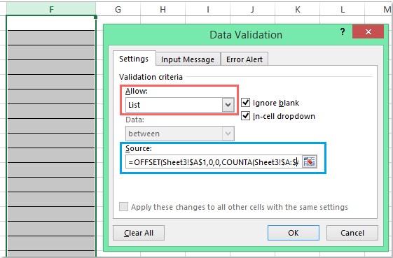
1. Izberite celice, kamor želite vstaviti spustni seznam, in kliknite datum > Preverjanje podatkov > Preverjanje podatkov, glej posnetek zaslona:

doc spustni seznam privzeto na vrh 2

2. V izskočil Preverjanje podatkov v pogovornem oknu pod Nastavitve izberite jeziček Seznam Iz Dovoli in vnesite to formulo: = OFFSET (Sheet3! $ A $ 1,0,0, COUNTA (Sheet3! $ A: $ A) -1,1) v vir besedilno polje, glej posnetek zaslona:

Opombe: V tej formuli, Sheet3 je delovni list vsebuje seznam izvornih podatkov in A1 je prva vrednost celice na seznamu.

doc spustni seznam privzeto na vrh 3

3. Nato kliknite OK Ko kliknete celice spustnega seznama, je prvi podatkovni element vedno prikazan na vrhu, ali so na koncu izvornih podatkov izbrisane vrednosti celic, glejte posnetek zaslona:

doc spustni seznam privzeto na vrh 4


puščica modri desni mehurček Samodejno prikaži prvi element na spustnem seznamu, namesto prazen s kodo VBA

Tu lahko predstavim tudi kodo VBA, s katero lahko samodejno prikažete prvi element na spustnem seznamu, ko kliknete celice za preverjanje veljavnosti podatkov.

1. Po vstavitvi spustnega seznama izberite zavihek delovnega lista, ki vsebuje spustni seznam, in z desno miškino tipko izberite Ogled kode iz kontekstnega menija, da odprete Microsoft Visual Basic za aplikacije okno in nato v modul kopirajte in prilepite naslednjo kodo:

Koda VBA: Samodejno prikaži prvi podatkovni element na spustnem seznamu:

Private Sub Worksheet_SelectionChange(ByVal Target As Range)
'Updateby Extendoffice 20160725
    Dim xFormula As String
    On Error GoTo Out:
    xFormula = Target.Cells(1).Validation.Formula1
    If Left(xFormula, 1) = "=" Then
        Target.Cells(1) = Range(Mid(xFormula, 1)).Cells(1).Value
    End If
Out:
End Sub

doc spustni seznam privzeto na vrh 5

2. Nato shranite in zaprite okno s kodo, in zdaj, ko kliknete celico spustnega seznama, bo hkrati prikazan prvi podatkovni element.

Najboljša pisarniška orodja za produktivnost

🤖 Kutools AI Aide: Revolucionirajte analizo podatkov na podlagi: Inteligentna izvedba   |  Ustvari kodo  |  Ustvarite formule po meri  |  Analizirajte podatke in ustvarite grafikone  |  Prikličite funkcije Kutools...
Priljubljene funkcije: Poiščite, označite ali identificirajte dvojnike   |  Izbriši prazne vrstice   |  Združite stolpce ali celice brez izgube podatkov   |   Krog brez formule ...
Super iskanje: Več kriterijev VLookup    Multiple Value VLookup  |   VLookup na več listih   |   Nejasno iskanje ....
Napredni spustni seznam: Hitro ustvarite spustni seznam   |  Odvisni spustni seznam   |  Večkrat izberite spustni seznam ....
Upravitelj stolpcev: Dodajte določeno število stolpcev  |  Premakni stolpce  |  Preklop stanja vidnosti skritih stolpcev  |  Primerjaj obsege in stolpce ...
Predstavljene funkcije: Mrežni fokus   |  Pogled oblikovanja   |   Velika vrstica formule    Upravitelj delovnih zvezkov in listov   |  Knjižnica virov (Samodejno besedilo)   |  Izbirnik datuma   |  Združite delovne liste   |  Šifriranje/dešifriranje celic    Pošljite e-pošto po seznamu   |  Super filter   |   Poseben filter (filter krepko/ležeče/prečrtano ...) ...
15 najboljših kompletov orodij12 Besedilo Orodja (dodajanje besedila, Odstrani znake,...)   |   50 + Graf Vrste (Gantt Chart,...)   |   40+ Praktično Formule (Izračunajte starost glede na rojstni dan,...)   |   19 vstavljanje Orodja (Vstavite kodo QR, Vstavi sliko s poti,...)   |   12 Pretvorba Orodja (Številke v besede, Pretvorba valut,...)   |   7 Spoji in razdeli Orodja (Napredne kombinirane vrstice, Razdeljene celice,...)   |   ... in več

Napolnite svoje Excelove spretnosti s Kutools za Excel in izkusite učinkovitost kot še nikoli prej. Kutools za Excel ponuja več kot 300 naprednih funkcij za povečanje produktivnosti in prihranek časa.  Kliknite tukaj, če želite pridobiti funkcijo, ki jo najbolj potrebujete...

Opis


Kartica Office prinaša vmesnik z zavihki v Office in poenostavi vaše delo

  • Omogočite urejanje in branje z zavihki v Wordu, Excelu, PowerPointu, Publisher, Access, Visio in Project.
  • Odprite in ustvarite več dokumentov v novih zavihkih istega okna in ne v novih oknih.
  • Poveča vašo produktivnost za 50%in vsak dan zmanjša na stotine klikov miške za vas!
Comments (10)
No ratings yet. Be the first to rate!
This comment was minimized by the moderator on the site
=OFFSET(Sheet3!$A$1,0,0,COUNTA(Sheet3!$A:$A)+2-1,1) I added +2 to the equation and that worked for me.
This comment was minimized by the moderator on the site
For the VDA code, how can I have only a certain cell range show the first item in the drop down list? Thank you in advance.
This comment was minimized by the moderator on the site
Hi, Akrupa,To solve your problem, maybe the following VBA code can help you:

<div data-tag="code">Private Sub Worksheet_SelectionChange(ByVal Target As Range)
'Updateby Extendoffice 20211206
Dim xFormula As String
Dim xRg As Range
Dim xStr As String
Dim xIndex As Integer
xIndex = 2 'Here indicates the cell number of the original data,for example,the original data is A1:A10, to display the A2 cell value, please write 2 here.
On Error GoTo Out:
xFormula = Target.Cells(1).Validation.Formula1
If Left(xFormula, 1) = "=" Then
If Target.Value <> "" Then Exit Sub
xStr = Mid(xFormula, 2)
Set xRg = Application.Range(xStr)
Target.Cells(1) = xRg.Cells(xIndex).Value
End If
Out:
End Sub
Please try, hope it can help you!
This comment was minimized by the moderator on the site
Better but not quite. Using the =OFFSET(Sheet3!$A$1,0,0,COUNTA(Sheet3!$A:$A)-1,1) method eliminates the blanks but still starts you at the bottom of the very long list. I want it to start at the top of the list.
This comment was minimized by the moderator on the site
Once again, you save the day! Thanks!
This comment was minimized by the moderator on the site
Doesn't work for me. I keep getting an error message that says, "There's a problem with this formula. Not trying to type a formula? When the first character is an equal (+) or minus (-) sign, Exel thinks it's a formula.... To get around this, type an apostrophe (') first..."
This comment was minimized by the moderator on the site
Hello!

How can I set a data validation list such that if the drop down value in the cell is deleted, the cell will automatically show a default value (i.e. "-Select-")?

For example, I have a worksheet with multiple drop down lists that I want to show a default value of "-Select-" once the sheet is opened. A user will select values from the lists that will impact the result of calculations throughout the entire spreadsheet. A user may accidentally "delete" the cell contents of the lists. If this happens, rather than the cell becoming blank, I want the cell to show a default value of "-Select-". This scenario occurs in multiple random locations throughout the spreadsheet, not just in one localized place.

I was able to find the following VBA code so far, but it only applies the concept over a range, rather than just individual cells that contain drop down lists. The problem with what I have coded so far is that every single blank cell in the range ends up with "-Select-" in it. Some of the lists are in ranges, but some are also scattered throughout the sheet. The problem I'm having with my current code is that every single blank cell in the range ends up with "-Select-" in it. I'm trying to get this to apply over the entire worksheet to ONLY cells that are drop down lists.

Is what I'm trying to accomplish even possible?

Example file can be found here:
https://drive.google.com/file/d/1VoO8VgFs3IJ0ALwqfk0i8gt69UE4vEKW/view?usp=sharing

Example code:

Option Explicit

Private Sub Worksheet_Change(ByVal Target As Range)
Dim cel As Range
' If Target.Cells.Count > 1 Then Exit Sub 'turning this off allows multiple cells to be selected and deleted at the same time
If Not Intersect(Target, Range("f2:p17")) Is Nothing Then
For Each cel In Range("f2:p17")
Application.EnableEvents = False
If IsEmpty(cel.Value) Then cel.Value = "-Select-"
Next cel
End If
Application.EnableEvents = True
End Sub


Thanks in advance!
This comment was minimized by the moderator on the site
How can I set a data validation list such that if the drop down value in the cell is deleted, the cell will automatically show the a default value (i.e. "-Select-")?

For example, I have a worksheet with multiple drop down lists that I want to show a default value of "-Select-" once the sheet is opened. A user will select values from the lists that will impact the result of calculations throughout the entire spreadsheet. A user may accidentally "delete" the cell contents. If this happens, rather than the cell becoming blank, I want the cell to show a default value of "-Select-". This scenario occurs in multiple random locations throughout the spreadsheet, not just in one localized place.

I was able to come up with the following VBA code so far, but I've only figured out how to apply the concept over a range, rather than just cells that contain a drop down list. The problem with what I have coded so far is that every single blank cell in the range ends up with "-Select-" in it.

Option Explicit

Private Sub Worksheet_Change(ByVal Target As Range)
Dim cel As Range
' If Target.Cells.Count > 1 Then Exit Sub
If Not Intersect(Target, Range("f2:p17")) Is Nothing Then
For Each cel In Range("f2:p17")
Application.EnableEvents = False
If IsEmpty(cel.Value) Then cel.Value = "-Select-"
Next cel
End If
Application.EnableEvents = True
End Sub
This comment was minimized by the moderator on the site
select the cell in which you have put the listitem
the range for the listitem is "Opleiding"
in your VBA code:

selection.Value = Range("opleiding").Cells(2, 1)

the result is that the selected item of the listItem is the second item in the range "Opleiding"
This comment was minimized by the moderator on the site
After scroll down select to cells numeric data not come in series only first cell data come select 1,2 different cells and scroll down value not coming 1,2,3,4,5....... only first cell value coming 1,1,1,1,....
There are no comments posted here yet
Please leave your comments in English
Posting as Guest
×
Rate this post:
0   Characters
Suggested Locations