Preskoči na glavno vsebino

Kako posodobiti formulo pri vstavljanju vrstic v Excelu? 

doc posodobitev formule vstavljanje vrstic 1

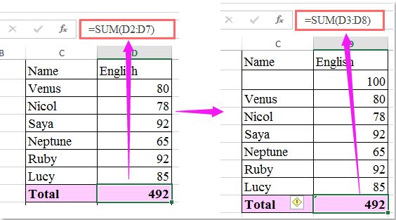
Na primer, v celici D2 imam formulo = vsota (D7: D8), zdaj, ko v drugo vrstico vstavim vrstico in vnesem novo številko, se formula samodejno spremeni v = vsota (D3: D8), kar izključi celico D2, kot je prikazano na sliki spodaj. V tem primeru moram vsakič, ko vstavim vrstice, spremeniti sklic na celico v formuli. Kako lahko pri vstavljanju vrstic v Excelu vedno seštevam številke, ki se začnejo od celice D2?

Posodobi formulo pri samodejnem vstavljanju vrstic s formulo


puščica modri desni mehurček Posodobi formulo pri samodejnem vstavljanju vrstic s formulo

Naslednja preprosta formula vam lahko pomaga samodejno posodobiti formulo, ne da bi pri vstavljanju novih vrstic ročno spreminjali sklic na celico, naredite naslednje:

1. Vnesite to formulo: = VSEBINA (POSREDNO ("D2: D" in RED () - 1)) (D2 je prva celica na seznamu, ki jo želite sešteti) na koncu celic, v katere želite sešteti seznam številk, in pritisnite Vnesite ključ.

2. In zdaj, ko kamor koli med seznam števil vstavite vrstice, se formula samodejno posodobi, glejte posnetek zaslona:

doc posodobitev formule vstavljanje vrstic 2

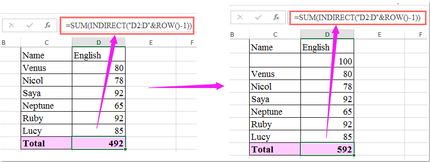
nasveti: Formula deluje pravilno le, če jo postavite na konec seznama podatkov.

Najboljša pisarniška orodja za produktivnost

🤖 Kutools AI Aide: Revolucionirajte analizo podatkov na podlagi: Inteligentna izvedba   |  Ustvari kodo  |  Ustvarite formule po meri  |  Analizirajte podatke in ustvarite grafikone  |  Prikličite funkcije Kutools...
Priljubljene funkcije: Poiščite, označite ali identificirajte dvojnike   |  Izbriši prazne vrstice   |  Združite stolpce ali celice brez izgube podatkov   |   Krog brez formule ...
Super iskanje: Več kriterijev VLookup    Multiple Value VLookup  |   VLookup na več listih   |   Nejasno iskanje ....
Napredni spustni seznam: Hitro ustvarite spustni seznam   |  Odvisni spustni seznam   |  Večkrat izberite spustni seznam ....
Upravitelj stolpcev: Dodajte določeno število stolpcev  |  Premakni stolpce  |  Preklop stanja vidnosti skritih stolpcev  |  Primerjaj obsege in stolpce ...
Predstavljene funkcije: Mrežni fokus   |  Pogled oblikovanja   |   Velika vrstica formule    Upravitelj delovnih zvezkov in listov   |  Knjižnica virov (Samodejno besedilo)   |  Izbirnik datuma   |  Združite delovne liste   |  Šifriranje/dešifriranje celic    Pošljite e-pošto po seznamu   |  Super filter   |   Poseben filter (filter krepko/ležeče/prečrtano ...) ...
15 najboljših kompletov orodij12 Besedilo Orodja (dodajanje besedila, Odstrani znake,...)   |   50 + Graf Vrste (Gantt Chart,...)   |   40+ Praktično Formule (Izračunajte starost glede na rojstni dan,...)   |   19 vstavljanje Orodja (Vstavite kodo QR, Vstavi sliko s poti,...)   |   12 Pretvorba Orodja (Številke v besede, Pretvorba valut,...)   |   7 Spoji in razdeli Orodja (Napredne kombinirane vrstice, Razdeljene celice,...)   |   ... in več

Napolnite svoje Excelove spretnosti s Kutools za Excel in izkusite učinkovitost kot še nikoli prej. Kutools za Excel ponuja več kot 300 naprednih funkcij za povečanje produktivnosti in prihranek časa.  Kliknite tukaj, če želite pridobiti funkcijo, ki jo najbolj potrebujete...

Opis


Kartica Office prinaša vmesnik z zavihki v Office in poenostavi vaše delo

  • Omogočite urejanje in branje z zavihki v Wordu, Excelu, PowerPointu, Publisher, Access, Visio in Project.
  • Odprite in ustvarite več dokumentov v novih zavihkih istega okna in ne v novih oknih.
  • Poveča vašo produktivnost za 50%in vsak dan zmanjša na stotine klikov miške za vas!
Comments (9)
No ratings yet. Be the first to rate!
This comment was minimized by the moderator on the site
Thank you very much.
This comment was minimized by the moderator on the site
Hello,
You are welcome. Glad it helps. Any questions, please feel free to contact us. Have a great day.
Sincerely,
Mandy
This comment was minimized by the moderator on the site
Please help me with Excel formula that update automatically without changing the cell reference manually when inserting new row at the bottom only. But not when inserting new row at the top. Thanks
This comment was minimized by the moderator on the site
This is really helpful ... except it does not update the row/column when copying and pasting this formula, so if I have a bunch of them, I have to update the column/row manually (like in the example, if I copy this to the adjacent column E, it still has D ...)

Unless someone knows a workaround to that problem, too?
This comment was minimized by the moderator on the site
you can use a different formula SUM(D$2:D12) as you insert a new row it continues to sum it up
This comment was minimized by the moderator on the site
I found that this only works if there is more than 1 row to total at the start.  Any ideas how you would do this for totalling 1 row to start and then adding in rows as you work on the spreadsheet?

This comment was minimized by the moderator on the site
You are the best! It works!
This comment was minimized by the moderator on the site
I have a simple cell reference in one of my cells down a column e.g.:"=H6", “=H7” etc. When I insert a row in Excel and copy formulas from row above, the cell reference in 'Opening Stock' does not update automatically in the row after the new blank row (should be equal to previous row balance, which is 60 now). But it updates correctly in all other rows below. Is there a way to force Excel to update cell reference to the cell in blank row above? Have searched the web, but did not get any satisfactory answer. I do not want to convert the data to a table, since it messes up the filters and formatting. Macros don't solve the problem either - they don't copy to the row following the blank one. Can anyone please help?
This comment was minimized by the moderator on the site
Hi Rayan!

Please if you see this let me know! You are the only one I found online who brought this issue up. However, my data is table not normal range. The automatic filling of the formula really helps and copy/pasting is a hassle. Anyway, when insert a row, the formulas update for all columns except one! In the row and the cell, instead of the formula shifting from =if(C24 = C25) to =if(C25 = C26), it goes to =if(C24 = C26) although C24 is not fixed!!! I've really tried all possible solutions...................
There are no comments posted here yet
Please leave your comments in English
Posting as Guest
×
Rate this post:
0   Characters
Suggested Locations