Preskoči na glavno vsebino

Kako ustvariti odvisen spustni seznam v Googlovem listu?

Vstavljanje običajnega spustnega seznama v Googlov list je za vas lahko enostavno, včasih pa boste morda morali vstaviti odvisen spustni seznam, kar pomeni drugi spustni seznam, odvisno od izbire prvega spustnega seznama. Kako bi se lahko spoprijeli s to nalogo v Googlovem listu?

Ustvarite odvisen spustni seznam v Googlovem listu


Ustvarite odvisen spustni seznam v Googlovem listu

Naslednji koraki vam bodo morda pomagali pri vstavljanju odvisnega spustnega seznama. Naredite naslednje:

1. Najprej vstavite osnovni spustni seznam, izberite celico, kamor želite postaviti prvi spustni seznam, in nato kliknite datum > Validacija podatkov, glej posnetek zaslona:

2. V izskočil Validacija podatkov pogovorno okno, izberite Seznam iz obsega s spustnega seznama ob Merila in nato kliknite gumb, da izberete vrednosti celic, na podlagi katerih želite ustvariti prvi spustni seznam, glejte posnetek zaslona:

3. Nato kliknite Shrani gumb, je bil ustvarjen prvi spustni seznam. Na ustvarjenem spustnem seznamu izberite en element in nato vnesite to formulo: =arrayformula(if(F1=A1,A2:A7,if(F1=B1,B2:B6,if(F1=C1,C2:C7,"")))) v prazno celico, ki meji na stolpce s podatki, nato pritisnite Vnesite ključ, so bile naenkrat prikazane vse ujemajoče se vrednosti na podlagi prvega elementa spustnega seznama, glejte posnetek zaslona:

Opombe: V zgornji formuli: F1 je prva celica spustnega seznama, A1, B1 in C1 so elementi prvega spustnega seznama, A2: A7, B2: B6 in C2: C7 so vrednosti celic, na katerih temelji drugi spustni seznam. Lahko jih spremenite v svoje.

4. Nato lahko ustvarite drugi odvisni spustni seznam, kliknite celico, kamor želite dodati drugi spustni seznam, in nato kliknite datum > Validacija podatkov Pojdite na Validacija podatkov izberite pogovorno okno Seznam iz obsega od spustnega menija ob Merila in kliknite gumb, da izberete celice formule, ki so ujemajoči se rezultati prvega spustnega elementa, glejte posnetek zaslona:

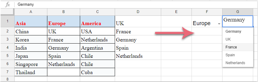
5. Končno kliknite gumb Shrani in drugi odvisni spustni seznam je bil uspešno ustvarjen, kot je prikazano na sliki spodaj:

Najboljša pisarniška orodja za produktivnost

🤖 Kutools AI Aide: Revolucionirajte analizo podatkov na podlagi: Inteligentna izvedba   |  Ustvari kodo  |  Ustvarite formule po meri  |  Analizirajte podatke in ustvarite grafikone  |  Prikličite funkcije Kutools...
Priljubljene funkcije: Poiščite, označite ali identificirajte dvojnike   |  Izbriši prazne vrstice   |  Združite stolpce ali celice brez izgube podatkov   |   Krog brez formule ...
Super iskanje: Več kriterijev VLookup    Multiple Value VLookup  |   VLookup na več listih   |   Nejasno iskanje ....
Napredni spustni seznam: Hitro ustvarite spustni seznam   |  Odvisni spustni seznam   |  Večkrat izberite spustni seznam ....
Upravitelj stolpcev: Dodajte določeno število stolpcev  |  Premakni stolpce  |  Preklop stanja vidnosti skritih stolpcev  |  Primerjaj obsege in stolpce ...
Predstavljene funkcije: Mrežni fokus   |  Pogled oblikovanja   |   Velika vrstica formule    Upravitelj delovnih zvezkov in listov   |  Knjižnica virov (Samodejno besedilo)   |  Izbirnik datuma   |  Združite delovne liste   |  Šifriranje/dešifriranje celic    Pošljite e-pošto po seznamu   |  Super filter   |   Poseben filter (filter krepko/ležeče/prečrtano ...) ...
15 najboljših kompletov orodij12 Besedilo Orodja (dodajanje besedila, Odstrani znake,...)   |   50 + Graf Vrste (Gantt Chart,...)   |   40+ Praktično Formule (Izračunajte starost glede na rojstni dan,...)   |   19 vstavljanje Orodja (Vstavite kodo QR, Vstavi sliko s poti,...)   |   12 Pretvorba Orodja (Številke v besede, Pretvorba valut,...)   |   7 Spoji in razdeli Orodja (Napredne kombinirane vrstice, Razdeljene celice,...)   |   ... in več

Napolnite svoje Excelove spretnosti s Kutools za Excel in izkusite učinkovitost kot še nikoli prej. Kutools za Excel ponuja več kot 300 naprednih funkcij za povečanje produktivnosti in prihranek časa.  Kliknite tukaj, če želite pridobiti funkcijo, ki jo najbolj potrebujete...

Opis


Kartica Office prinaša vmesnik z zavihki v Office in poenostavi vaše delo

  • Omogočite urejanje in branje z zavihki v Wordu, Excelu, PowerPointu, Publisher, Access, Visio in Project.
  • Odprite in ustvarite več dokumentov v novih zavihkih istega okna in ne v novih oknih.
  • Poveča vašo produktivnost za 50%in vsak dan zmanjša na stotine klikov miške za vas!
Comments (18)
No ratings yet. Be the first to rate!
This comment was minimized by the moderator on the site
Hi there. Its been working but for it only appears that only one cell can be formulated.I need help 
For example: in Cell A1, it shows dependent dropdown, but when in cell a2 it does not work.
Thas what help that i need, From A:A, They have all different selection from the dropdown list. Thanks.
This comment was minimized by the moderator on the site
Would it been possible to create pull down menu based of formula?
I use formula "=SUMIFS(Items!$I:$I,Items!$A:$A,K$1,Items!$D:$D,$D2)" (=for example 150) to find the qty on pallet based on item and container size.
So I wanted to create pull down menu like qty 1 pallet, qty 2 pallets, qty 3 pallets,.....
Then user will always order qty of full pallets like 150, 2 x 150, 3 x150, up to 21 x 150.
This comment was minimized by the moderator on the site
Hi, I already created a drop down list like this one, what I'd like to know is how i can, when clicking on one option from that list, restrict what appears as options on another cell. For example, in one cell i can choose between laparoscopy and orthopaedics. If I choose orthopaedics then, the other cell which has a list of doctors, should only show the doctors for orthopedy and not all of them. Does anyone know how to do this?
This comment was minimized by the moderator on the site
Hii Sir,
I Want to Create A Dependent Drop Down List Like
- State(A1):- District(B1):- Taluka(C1) :- Then Information(D1) ,
So I need your Help .
Tell How do you do this Type of Dependent Drop down List in Excel or Google Sheet
This comment was minimized by the moderator on the site
Hi, Shelate,
Maybe the below article can solve your problem, please view it:
https://www.extendoffice.com/documents/excel/5852-excel-multiple-level-drop-down-list.html

Please try, hope it can help you!
This comment was minimized by the moderator on the site
Now is needed to use: =arrayformula(if(F1=A1;A2:A7;if(F1=B1;B2:B6;if(F1=C1;C2:C7;""))))
This comment was minimized by the moderator on the site
Thank you soooo much!
This comment was minimized by the moderator on the site
Hi,
I was wondering if anyone could advise me with this? I've followed the above steps but on step 3 rather than getting:
"...all the matching values based on the first drop down list item have been displayed at once," I am just seeing one value (the top one from the drop down list).
My cells are placed slightly differently and the first drop down is filled from another sheet (from anywhere int eh column excluding the top row) so my formula is:

=arrayformula(if(VLE!D2:D=B11,B12,if(VLE!D2:D=C11,C12:C14,if(VLE!D2:D=D11,D12:D14,if(VLE!D2:D=E11,E12:E16,if(VLE!D2:D=F11,F12:F16,""))))))

It is correctly displaying the top drop down option for each of (using cell numbers from the step 3 example on this page) A1, B1, and C1 so, again using this page's example, if I select Asia form the F1 drop down, I would get China, but nothing further


Any suggestions?

Many thanks! Nick
This comment was minimized by the moderator on the site
If the first drop own is on sheet 1 A1, will this work were I want the second drop down as sheet 1 A2, but to have its data range on a separate sheet?
This comment was minimized by the moderator on the site
Ich bekomm immer die Meldung "Fehler beim Parsen der Formel" wenn ich =arrayformula(if(F1=A1,A2:A7,if(F1=B1,B2:B6,if(F1=C1,C2:C7,"")))) eingebe. Was ist der "Weiter-Schlüsel"? Reicht es nicht wie bei Excel die Formel einzugeben?
This comment was minimized by the moderator on the site
Ersetzen Sie den , zu ;
es hat für mich funktioniert
This comment was minimized by the moderator on the site
This is the best explanation I have found, so thank you for that!

In my situation, I am working with over 200 rows with more being continuously added. Is there an easier/more efficient way to handle this many rows?
This comment was minimized by the moderator on the site
Yes, if you don't put number index to specify ending cell.
Like instead of C2:C7 you put C2:C. This will automatically tell the array formula, that you want to consider all values in column "C" starting at "C2".
This comment was minimized by the moderator on the site
What happens if I want exactly the same dropdown list in F2 as you have in F1 ?
I tried, and it doesn't overwrite D1:D7 .. meaning D1:D7 is only available once.
I need something else, double dropdown, but on many-many lines .. guess I must use another system then .. not sure which ..
This comment was minimized by the moderator on the site
Hi, Xained,
This method can only applied to one cell, if you have some good ways for applying this to multiple cells, please comment here.

Thank you!
This comment was minimized by the moderator on the site
Please, guide me how to do that.Thanks
This comment was minimized by the moderator on the site
혹시, 하나의 셀이 아닌 여러셀에 할 수 있는 방법을 알 수 있을까요?
This comment was minimized by the moderator on the site
내말이... 시바 좃빠지게 따라했디만 밑에줄은 안되노..
There are no comments posted here yet
Please leave your comments in English
Posting as Guest
×
Rate this post:
0   Characters
Suggested Locations