Preskoči na glavno vsebino

Kako pogojno oblikovanje na podlagi drugega lista v Googlovem listu?

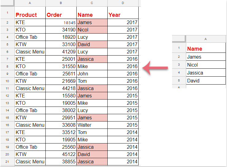
Če želite uporabiti pogojno oblikovanje, da označite celice na podlagi seznama podatkov z drugega lista, kot je prikazano na sliki zaslona, ​​prikazani na Googlovem listu, ali imate kakšne enostavne in dobre metode za njihovo reševanje?

Pogojno oblikovanje za označevanje celic na podlagi seznama z drugega lista v Google Preglednicah


Pogojno oblikovanje za označevanje celic na podlagi seznama z drugega lista v Google Preglednicah


Za dokončanje tega dela naredite naslednje:

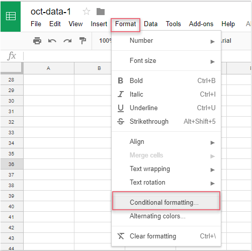
1. Kliknite oblikovana > Pogojno oblikovanje, glej posnetek zaslona:

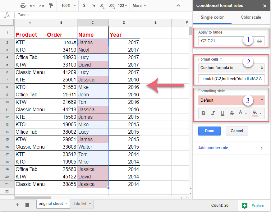
2. v Pravila pogojne oblike podokno, naredite naslednje:

(1.) Kliknite gumb, da izberete podatke stolpca, ki jih želite označiti;

(2.) V Oblikuj celice, če spustnega seznama, izberite Formula po meri je in nato vnesite to formulo: = ujemanje (C2, posredno ("seznam podatkov! A2: A"), 0) v besedilno polje;

(3.) Nato izberite eno obliko Stil oblikovanja kot jo potrebujete.

Opombe: V zgornji formuli: C2 je prva celica podatkov stolpca, ki jo želite označiti, in seznam podatkov! A2: A je obseg imena lista in seznama celic, ki vsebuje merila, na podlagi katerih želite poudariti celice.

3. In vse ujemajoče se celice, ki temeljijo na celicah s seznama, so bile hkrati označene, nato kliknite Done , da zaprete Pravila pogojne oblike podokno, kot ga potrebujete.


Najboljša pisarniška orodja za produktivnost

🤖 Kutools AI Aide: Revolucionirajte analizo podatkov na podlagi: Inteligentna izvedba   |  Ustvari kodo  |  Ustvarite formule po meri  |  Analizirajte podatke in ustvarite grafikone  |  Prikličite funkcije Kutools...
Priljubljene funkcije: Poiščite, označite ali identificirajte dvojnike   |  Izbriši prazne vrstice   |  Združite stolpce ali celice brez izgube podatkov   |   Krog brez formule ...
Super iskanje: Več kriterijev VLookup    Multiple Value VLookup  |   VLookup na več listih   |   Nejasno iskanje ....
Napredni spustni seznam: Hitro ustvarite spustni seznam   |  Odvisni spustni seznam   |  Večkrat izberite spustni seznam ....
Upravitelj stolpcev: Dodajte določeno število stolpcev  |  Premakni stolpce  |  Preklop stanja vidnosti skritih stolpcev  |  Primerjaj obsege in stolpce ...
Predstavljene funkcije: Mrežni fokus   |  Pogled oblikovanja   |   Velika vrstica formule    Upravitelj delovnih zvezkov in listov   |  Knjižnica virov (Samodejno besedilo)   |  Izbirnik datuma   |  Združite delovne liste   |  Šifriranje/dešifriranje celic    Pošljite e-pošto po seznamu   |  Super filter   |   Poseben filter (filter krepko/ležeče/prečrtano ...) ...
15 najboljših kompletov orodij12 Besedilo Orodja (dodajanje besedila, Odstrani znake,...)   |   50 + Graf Vrste (Gantt Chart,...)   |   40+ Praktično Formule (Izračunajte starost glede na rojstni dan,...)   |   19 vstavljanje Orodja (Vstavite kodo QR, Vstavi sliko s poti,...)   |   12 Pretvorba Orodja (Številke v besede, Pretvorba valut,...)   |   7 Spoji in razdeli Orodja (Napredne kombinirane vrstice, Razdeljene celice,...)   |   ... in več

Napolnite svoje Excelove spretnosti s Kutools za Excel in izkusite učinkovitost kot še nikoli prej. Kutools za Excel ponuja več kot 300 naprednih funkcij za povečanje produktivnosti in prihranek časa.  Kliknite tukaj, če želite pridobiti funkcijo, ki jo najbolj potrebujete...

Opis


Kartica Office prinaša vmesnik z zavihki v Office in poenostavi vaše delo

  • Omogočite urejanje in branje z zavihki v Wordu, Excelu, PowerPointu, Publisher, Access, Visio in Project.
  • Odprite in ustvarite več dokumentov v novih zavihkih istega okna in ne v novih oknih.
  • Poveča vašo produktivnost za 50%in vsak dan zmanjša na stotine klikov miške za vas!


Comments (27)
Rated 5 out of 5 · 2 ratings
This comment was minimized by the moderator on the site
Hi! skyyang ! Thank you, =match(C2,indirect("data list!A2:A"),0) works for me.

But I would like to format more than one column, so column A in sheet a is checked against column B in sheet b , and so.
There are so many columns so I can not apply one format per column, but a whole conditional format for the whole sheet.


How should I modify the range and the formula?

Thanks!
This comment was minimized by the moderator on the site
What if the cell values you're trying to match are hyperlinks?
Rated 5 out of 5
This comment was minimized by the moderator on the site
Pardon, il fallait lire =A1<>INDIRECT("PreviousVersion!"& CHAR (COLUMN () + 64) & ROW ()) ...
This comment was minimized by the moderator on the site
Bonjour,
J'ai une autre question du même type au sujet d'un formatage conditionnel qui fonctionne sur Excel mais que je n'arrive pas à porter sur Google Sheet :
L'idée est de comparer 2 versions d'une même feuille que l'on stock à l'aide de 2 onglets (2 feuilles du même workbook)

La formule est la suivante : =A1<>'previousVersion'!A1 avec un formatage fond jaune pour mettre en évidence les changements sur toute la feuille car l'idée est d'appliquer ce
formatage conditionnel sur toutes les cellules de la feuille ($A$1:$V:1000)

Sur Google sheet cette formule m'est interdite et si je passe par un "indirect("previousVersion!A1"), je perds le coté dynamique sur le "A1" de la feuille precious version
Si j'essaye =A1<>indirect("previousVersion!"&A1) j'ai une erreur car c'est la valeur de A1 qui est interprétée et concaténée avec "previousVersion!"

Si j'essaye la formule =C3<>INDIRECT("PreviousVersion!"& CHAR (COLUMN () + 64) & ROW ()) cela ne fonctionne pas non plus....

Si vous avez une solution...
Merci d'avance
This comment was minimized by the moderator on the site
Bonjour,
Dans Feuille google je cherche la formule suivante
Si dans la cel A1 = text alors dans la Cel B1 ecire telle valeur ou texte automatiquement
Merci d avance pour votre aide
This comment was minimized by the moderator on the site
What if it's not an exact match but contains the reference data.
This comment was minimized by the moderator on the site
Hello, ashley
To solve your problem, please apply the below formula:
=REGEXMATCH(C2:C21,INDIRECT("Sheet2!$A$2"))

Please try, hope it can help you!
This comment was minimized by the moderator on the site
What happens if the data in my list is in more than one column? When I try to use datalist!A2:M or datalist!A:M or datalist!A2:M17 none of those work.
This comment was minimized by the moderator on the site
I have even tried naming the specific range I want to refer to and using that in the formula, no luck.
This comment was minimized by the moderator on the site
How to highlight the entire row data with conditional formatting using other sub-sheet
This comment was minimized by the moderator on the site
Hello, Ranganath
To highlight the entire row based on the data list, please do as this:
1. In the Apply to range box, select the whole sheet;
2. Apply this formula: =match($C2,indirect("datalist!A2:A"),0) into the Custom formula is textbox.
Please try, hope it can help you!

https://www.extendoffice.com/images/stories/comments/comment-skyyang/doc-highlight-entire-row.png
This comment was minimized by the moderator on the site
Hey, Thanks for replying. I have tried the formula but its not working.
Rated 5 out of 5
This comment was minimized by the moderator on the site
Hi,
Have you modified the sheet name and cell reference to your own data?
$C2 is the first cell of the column data that you want to highlight, and the datalist!A2:A is another sheet name and list range which contains the criteria you want to highlight the cells based on.
Please check them, thank you!
This comment was minimized by the moderator on the site
This doesn't work for me. I have triple checked everything.

Apply to range: K1:K2158

=match(K2,indirect("TorontoCitys!A1:A"),0)

It highlights random other city names, not in the TorontoCity's list.

K2 (is my main sheet and the starting column cell of the column I want to be affected.
TorontoCitys (is the name of the sheet)
A1 is the start of the column of the list of city names.
A is the column.

Could be that my punctuation's are incorrect?

Thanks in advance.
This comment was minimized by the moderator on the site
Hello friend,

Glad to help. Your formula is correct, please don't worry. The problem is the range you apply to. It shouldn't be K1:K2158, but K2:K2158.

Please see the screenshots. The example is simple but enough to explain the problem.

The correct "Apply to Range" is A2:A20. And the correct formula is =match(A2,indirect("TorontoCitys!A1:A"),0). Then correct cities can be highlighted. Please see screenshot 2.
But if I change the "Apply to Range" to A1:A20, the wrong city name is highlighted. Please see screenshot 3.

So please change your "Apply to Range" from K1:K2158 to K2:K2158. The problem should be solved. Looking forward to your reply.

Sincerely,
Mandy
This comment was minimized by the moderator on the site
how do you do this but with the entire row highlighted
There are no comments posted here yet
Load More
Please leave your comments in English
Posting as Guest
×
Rate this post:
0   Characters
Suggested Locations