Kako sumif celice, če vsebuje del besedilnega niza v listih Goolge?
Če želite v stolpcu sešteti vrednosti celic, če druge celice stolpcev vsebujejo del določenega besedilnega niza, kot je prikazano na sliki spodaj, bo ta članek predstavil nekaj uporabne formule za reševanje te naloge v Googlovih listih.
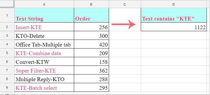
Sumif celice, če vsebuje del določenega besedilnega niza v Googlovih listih s formulami
Sumif celice, če vsebuje del določenega besedilnega niza v Googlovih listih s formulami
Naslednje formule vam lahko pomagajo pri seštevanju vrednosti celic, če celice drugih stolpcev vsebujejo določen besedilni niz, storite tako:
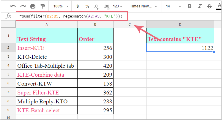
1. Vnesite to formulo: =sum(filter(B2:B9, regexmatch(A2:A9, "KTE"))) v prazno celico in pritisnite Vnesite tipko, da dobite rezultat, glejte sliko zaslona:
Opombe:
1. V zgornji formuli: B2: B9 je vrednost celic, ki jo želite sešteti, A2: A9 obseg vsebuje določen besedilni niz, "KTE"Je določeno besedilo, na podlagi katerega želite povzeti, spremenite jih glede na vaše potrebe.
2. Tu vam lahko pomaga tudi druga formula: =sumif(A2:A9,"*KTE*",B2:B9).
Najboljša pisarniška orodja za produktivnost
Napolnite svoje Excelove spretnosti s Kutools za Excel in izkusite učinkovitost kot še nikoli prej. Kutools za Excel ponuja več kot 300 naprednih funkcij za povečanje produktivnosti in prihranek časa. Kliknite tukaj, če želite pridobiti funkcijo, ki jo najbolj potrebujete...
")
Kartica Office prinaša vmesnik z zavihki v Office in poenostavi vaše delo
- Omogočite urejanje in branje z zavihki v Wordu, Excelu, PowerPointu, Publisher, Access, Visio in Project.
- Odprite in ustvarite več dokumentov v novih zavihkih istega okna in ne v novih oknih.
- Poveča vašo produktivnost za 50%in vsak dan zmanjša na stotine klikov miške za vas!
")