Negativna števila lahko spremenite v pozitivna z naslednjimi koraki:

1. Vnesite številko -1 v prazno celico, nato izberite to celico in pritisnite Ctrl + C tipke za kopiranje.

2. Izberite vsa negativna števila v obsegu, z desno miškino tipko kliknite in izberite Prilepi posebno ... iz kontekstnega menija. Oglejte si posnetek zaslona:

Opombe:
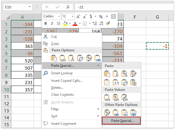
(1) Holding Ctrl tipko, lahko izberete vsa negativna števila, tako da jih kliknete eno za drugo;
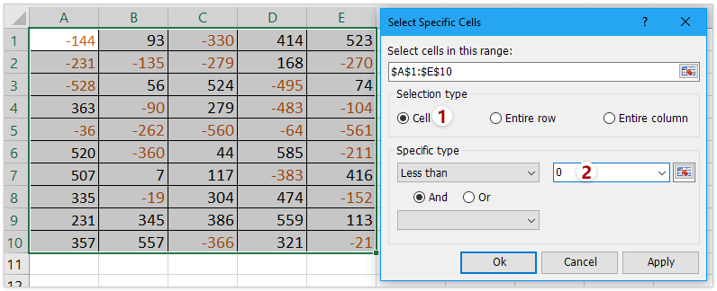
(2) Če imate nameščen Kutools za Excel, ga lahko uporabite Izberite Posebne celice funkcija za hitro izbiro vseh negativnih števil. Brezplačno preskusite!

3. In a Prilepite posebno prikaže se pogovorno okno, izberite vsi možnost od testeninetako, da izberete Pomnožite možnost od operacija, Kliknite OK. Oglejte si posnetek zaslona:

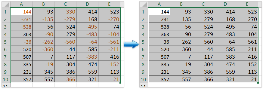
4. Vsa izbrana negativna števila bodo pretvorjena v pozitivna števila. Po potrebi izbrišite številko -1. Oglejte si posnetek zaslona:

Preprosto spremenite negativne številke na pozitivne v določenem obsegu v Excelu

V primerjavi z odstranjevanjem negativnega predznaka iz celic enega za drugim ročno, Kutools za Excel Spremeni znak vrednot funkcija omogoča izjemno enostaven način za hitro spreminjanje vseh negativnih številk v pozitivne pri izbiri. 30-dnevna popolna brezplačna preizkusna različica!

Kutools za Excel - Vključuje več kot 300 priročnih orodij za Excel. 30-dnevna brezplačna preizkusna različica brez kreditne kartice! Get It Now

Kot strokovnjak za Excel lahko tudi zaženete kodo VBA, da negativne številke spremenite v pozitivne številke.

1. Pritisnite tipki Alt + F11, da odprete okno Microsoft Visual Basic for Applications.

2. Prikazalo se bo novo okno. Kliknite Vstavi > Moduli, nato v modul vnesite naslednje kode:

Sub Positive
Dim Cel As Range
For Each Cel In Selection
If IsNumeric(Cel.Value) Then
Cel.Value = Abs(Cel.Value)
End If
Next Cel
End Sub

3. Nato kliknite Run ali pritisnite F5 tipka za zagon aplikacije in vsa negativna števila bodo spremenjena v pozitivna. Oglejte si posnetek zaslona:

Večina uporabnikov Excela ne želi uporabljati kode VBA, ali obstajajo hitri triki za spreminjanje negativnih števil v pozitivne? Kutools za excel vam lahko pomaga enostavno in udobno doseči to.

Kutools za Excel - Vključuje več kot 300 priročnih orodij za Excel. 30-dnevna brezplačna preizkusna različica brez kreditne kartice! Get It Now

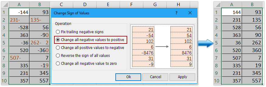
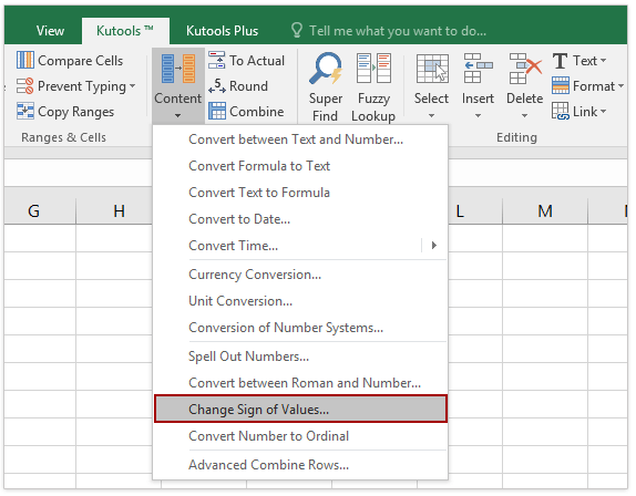
1. Izberite obseg, vključno z negativnimi števili, ki jih želite spremeniti, in kliknite Kutools > vsebina > Spremeni znak vrednot.

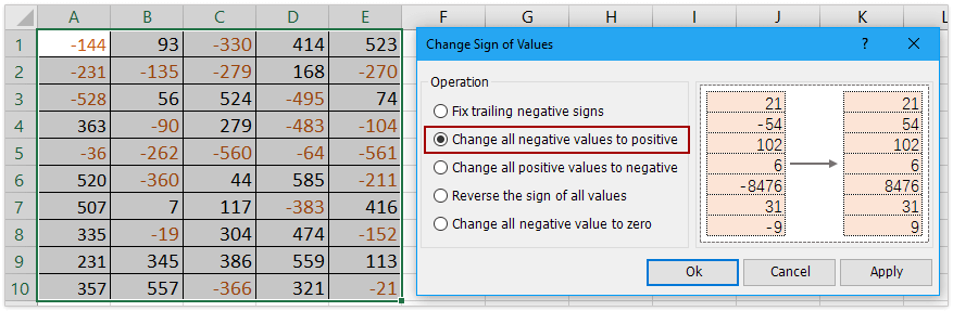
2. Check Spremenite vse negativne vrednosti na pozitivne pod operacijain kliknite Ok. Oglejte si posnetek zaslona:

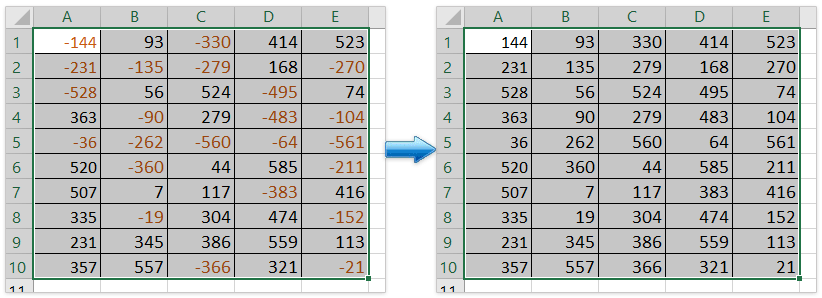
Zdaj boste videli, da se vsa negativna števila spremenijo v pozitivna, kot je prikazano spodaj:

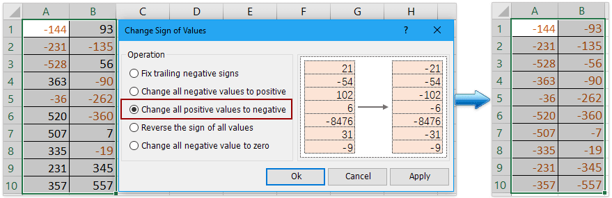
Opombe: S tem Spremeni znak vrednosti funkcijo, lahko tudi popravite negativne znake, spremenite vsa pozitivna števila v negativna, obrnete predznak vseh vrednosti in spremenite vse negativne vrednosti na nič. Brezplačno preskusite!

(1) Hitro spremenite vse pozitivne vrednosti na negativne v določenem obsegu:

(2) Preprosto obrnite znak vseh vrednosti v določenem obsegu:

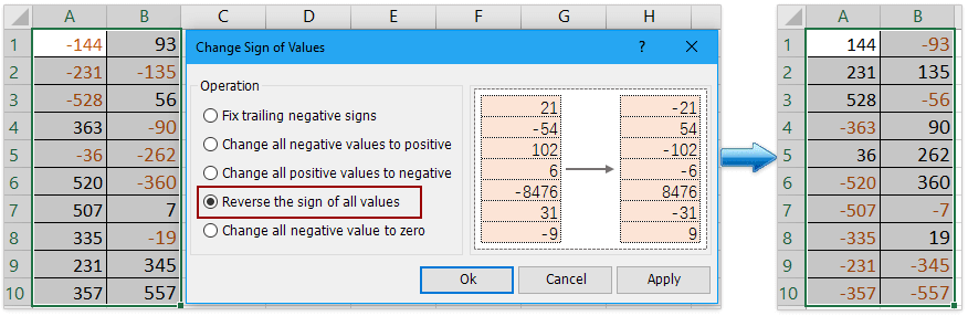
(3) Preprosto spremenite vse negativne vrednosti na nič v določenem obsegu:

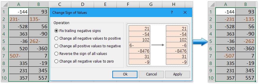
(4) Preprosto popravite negativne znake v določenem obsegu:

Kutools za Excel - Vključuje več kot 300 priročnih orodij za Excel. 30-dnevna brezplačna preizkusna različica brez kreditne kartice! Get It Now

Spremenite pozitivna števila v negativna

Obrnjeni znaki vrednosti v celicah

Popravite negativne znake v celicah

Spremenite negativno število na nič