Kako vrniti vrednost v drugi celici, če celica vsebuje določeno besedilo v Excelu?

Kot je prikazano v spodnjem primeru, ko celica E6 vsebuje vrednost »Da«, bo celica F6 samodejno napolnjena z vrednostjo »odobri«. Če spremenite »Da« v »Ne« ali »Nevtralnost« v E6, se vrednost v F6 takoj spremeni v »Zavrni« ali »Premisli«. Kako lahko storite, da ga dosežete? V tem članku je zbranih nekaj uporabnih metod, ki vam bodo pomagale enostavno rešiti težavo.

Vrni vrednost v drugi celici, če celica vsebuje določeno besedilo s formulo

Če želite vrniti vrednost v drugi celici, če celica vsebuje samo določeno besedilo, poskusite z naslednjo formulo. Če na primer B5 vsebuje "Da", vrnite "Odobri" v D5, drugače pa vrnite "Brez kvalifikacij". Naredite naslednje.

Izberite D5 in skopirajte spodnjo formulo vanjo ter pritisnite Vnesite tipko. Oglejte si posnetek zaslona:

Vrni vrednosti v drugi celici, če celica vsebuje različna besedila s formulo

Ta razdelek vam bo prikazal formulo za vrnitev vrednosti v drugi celici, če celica vsebuje drugačno besedilo v Excelu.

1. Ustvariti morate tabelo s posebnimi vrednostmi in vrnjenimi vrednostmi, ki se nahajajo ločeno v dveh stolpcih. Oglejte si posnetek zaslona:

2. Izberite prazno celico za vrnitev vrednosti, vanjo vnesite spodnjo formulo in pritisnite tipko Vnesite ključ, da dobite rezultat. Oglejte si posnetek zaslona:

Od zdaj naprej se bo pri spreminjanju vrednosti v E6 na določeno vrednost takoj vrnila v F6.

Enostavno vrnite vrednosti v drugi celici, če celica vsebuje drugačna besedila

Pravzaprav lahko zgornji problem rešite na lažji način. The Poiščite vrednost na seznamu uporabnost Kutools za Excel vam lahko pomaga, da ga dosežete z le nekaj kliki, ne da bi si zapomnili formulo.

1. Enako kot pri zgornji metodi morate tudi ustvariti tabelo s posebnimi vrednostmi in vrnjenimi vrednostmi, ki jih locirate ločeno v dveh stolpcih.

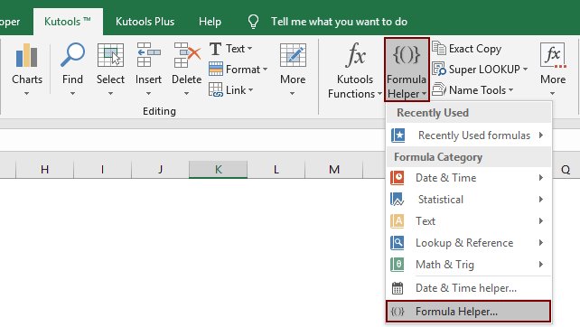
2. Izberite prazno celico, da izpišete rezultat (tukaj izberem F6), in kliknite Kutools > Pomočnik za formulo > Pomočnik za formulo. Oglejte si posnetek zaslona:

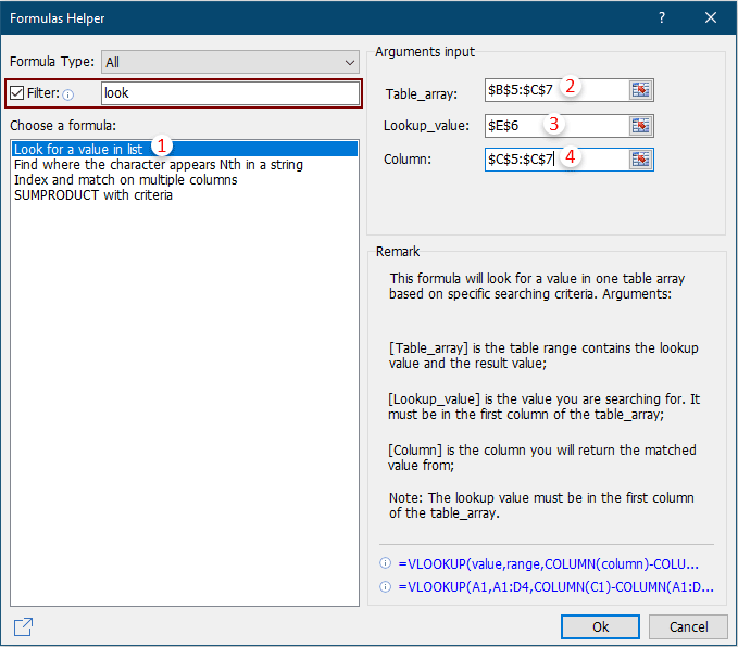
3. V Ljubljani Pomočnik za formulo pogovorno okno, nastavite na naslednji način:

• 3.1 V Izberite formulo poiščite in izberite Poiščite vrednost na seznamu;
  nasveti: Lahko preverite filter v polje za besedilo vnesite določeno besedo, da hitro filtrirate formulo.
• 3.2 V Tabela_ matrika izberite tabelo brez glav, ki ste jo ustvarili v 1. koraku;
• 3.2 V Iskalna_vrednost polje izberite polje vsebuje določeno vrednost, na podlagi katere boste vrnili vrednost;
• 3.3 V Stolpec v stolpcu določite stolpec, iz katerega boste vrnili ujemajočo se vrednost. Ali pa lahko v polje za besedilo vnesete številko stolpca neposredno, kot jo potrebujete.
• 3.4 Kliknite na OK . Oglejte si posnetek zaslona:

Od zdaj naprej se bo pri spreminjanju vrednosti v E6 na določeno vrednost takoj vrnila v F6. Glej rezultat kot spodaj:

Kutools za Excel - Pomaga vam, da vedno končate delo pred časom, imejte več časa za uživanje v življenju

Se pogosto znajdete v igri za dohitevanje dela, pomanjkanje časa zase in za družino?  Kutools za Excel vam lahko pomaga pri soočanju 80% Excel sestavljajo uganke in izboljšajo 80-odstotno delovno učinkovitost, dajo vam več časa za skrb za družino in uživanje v življenju.

300 naprednih orodij za 1500 delovnih scenarijev vam olajša delo kot kdaj koli prej.
Ni vam več treba zapomniti formul in kod VBA, odslej si privoščite počitek v možganih.
Zapletene in ponavljajoče se operacije je mogoče enkrat obdelati v nekaj sekundah.
Vsak dan zmanjšajte na tisoče operacij tipkovnice in miške, zdaj se poslovite od poklicnih bolezni.
Postanite strokovnjak za Excel v 3 minutah, vam pomaga hitro prepoznati in napredovanje za dvig plače.
Izbira 110,000 visoko učinkovitih ljudi in 300+ svetovno priznanih podjetij.
Naj bodo vaši 39.0 USD vredni več kot 4000.0 USD usposabljanja drugih.
Brezplačna preizkusna različica vseh funkcij 30-dan. 60-dnevna garancija vračila denarja brez razloga.