Preskoči na glavno vsebino

Kako se sklicevati na ime zavihka v celici v Excelu?

Avtor: Siluvia Zadnja sprememba: 2020-04-14

Za sklicevanje na trenutno ime zavihka lista v celici v Excelu lahko to storite s formulo ali uporabniško določeno funkcijo. Ta vadnica vas bo vodila na naslednji način.

Sklic na trenutno ime zavihka lista v celici s formulo
Sklicujte se na trenutno ime zavihka lista v celici z uporabniško določeno funkcijo
Kutools za Excel lahko preprosto sklicujete na trenutno ime zavihka lista v celici


Sklic na trenutno ime zavihka lista v celici s formulo

Navedite naslednje, da se sklicujete na ime aktivnega zavihka lista v določeni celici v Excelu.

1. Izberite prazno celico, kopirajte in prilepite formulo = MID (CELL ("ime datoteke", A1), FIND ("]", CELL ("ime datoteke", A1)) + 1,255) v vrstico formule in pritisnite Vnesite tipko. Oglejte si posnetek zaslona:

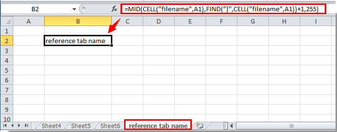
Zdaj se ime zavihka lista sklicuje v celici.

Preprosto vstavite ime zavihka v določeno celico, glavo ali nogo na delovnem listu:

O Kutools za Excel's Vstavite podatke o delovnem zvezku pripomoček pomaga enostavno vstaviti ime aktivnega zavihka v določeno celico. Poleg tega se lahko po potrebi sklicujete na ime delovnega zvezka, pot delovnega zvezka, uporabniško ime itd. V celico, glavo ali nogo delovnega lista. Kliknite za podrobnosti.
Prenesite Kutools za Excel zdaj! (30-dnevna brezplačna pot)


Sklicujte se na trenutno ime zavihka lista v celici z uporabniško določeno funkcijo

Poleg zgornje metode se lahko na ime zavihka lista v celici sklicujete s funkcijo User Define Function.

1. Pritisnite druga + F11 da odprete Microsoft Visual Basic za aplikacije okno.

2. V Ljubljani Microsoft Visual Basic za aplikacije okno, kliknite Vstavi > Moduli. Oglejte si posnetek zaslona:

3. Kopirajte in prilepite spodnjo kodo v okno Code. In nato pritisnite druga + Q tipke za zapiranje Microsoft Visual Basic za aplikacije okno.

Koda VBA: referenčno ime zavihka

Function TabName()
  TabName = ActiveSheet.Name
End Function

4. Pojdite v celico, v katero se želite sklicevati na ime trenutnega zavihka lista, vnesite = Ime zavihka () in nato pritisnite Vnesite tipko. Nato bo v celici prikazano ime trenutnega zavihka lista.


Sklicujte se na trenutno ime zavihka lista v celici s Kutools za Excel

Z Vstavite podatke o delovnem zvezku uporabnost Kutools za Excel, se lahko enostavno sklicujete na ime zavihka lista v poljubni celici. Naredite naslednje.

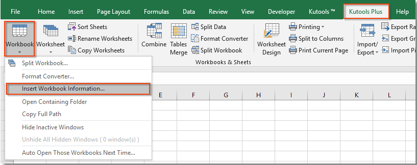
1. klik Kutools Plus > Delovni zvezek > Vstavite podatke o delovnem zvezku. Oglejte si posnetek zaslona:

2. V Ljubljani Vstavite podatke o delovnem zvezku pogovorno okno, izberite Ime delovnega lista v Informacije in v razdelku Vstavi pri izberete Območje in nato izberite prazno celico za iskanje imena lista in na koncu kliknite OK gumb.

Vidite lahko, da je trenutno ime lista sklicano na izbrano celico. Oglejte si posnetek zaslona:

  Če želite imeti brezplačno (30-dnevno) preskusno različico tega pripomočka, kliknite, če ga želite prenestiin nato nadaljujte z uporabo postopka v skladu z zgornjimi koraki.


Predstavitev: Kutools za Excel lahko preprosto sklicujete na ime trenutnega zavihka lista v celici

Kutools za Excel vključuje več kot 300 priročnih orodij Excel. Brezplačno poskusite brez omejitev v 30 dneh. Prenesite brezplačno preskusno različico zdaj!

Najboljša pisarniška orodja za produktivnost

🤖 Kutools AI Aide: Revolucionirajte analizo podatkov na podlagi: Inteligentna izvedba   |  Ustvari kodo  |  Ustvarite formule po meri  |  Analizirajte podatke in ustvarite grafikone  |  Prikličite funkcije Kutools...
Priljubljene funkcije: Poiščite, označite ali identificirajte dvojnike   |  Izbriši prazne vrstice   |  Združite stolpce ali celice brez izgube podatkov   |   Krog brez formule ...
Super iskanje: Več kriterijev VLookup    Multiple Value VLookup  |   VLookup na več listih   |   Nejasno iskanje ....
Napredni spustni seznam: Hitro ustvarite spustni seznam   |  Odvisni spustni seznam   |  Večkrat izberite spustni seznam ....
Upravitelj stolpcev: Dodajte določeno število stolpcev  |  Premakni stolpce  |  Preklop stanja vidnosti skritih stolpcev  |  Primerjaj obsege in stolpce ...
Predstavljene funkcije: Mrežni fokus   |  Pogled oblikovanja   |   Velika vrstica formule    Upravitelj delovnih zvezkov in listov   |  Knjižnica virov (Samodejno besedilo)   |  Izbirnik datuma   |  Združite delovne liste   |  Šifriranje/dešifriranje celic    Pošljite e-pošto po seznamu   |  Super filter   |   Poseben filter (filter krepko/ležeče/prečrtano ...) ...
15 najboljših kompletov orodij12 Besedilo Orodja (dodajanje besedila, Odstrani znake,...)   |   50 + Graf Vrste (Gantt Chart,...)   |   40+ Praktično Formule (Izračunajte starost glede na rojstni dan,...)   |   19 vstavljanje Orodja (Vstavite kodo QR, Vstavi sliko s poti,...)   |   12 Pretvorba Orodja (Številke v besede, Pretvorba valut,...)   |   7 Spoji in razdeli Orodja (Napredne kombinirane vrstice, Razdeljene celice,...)   |   ... in več

Napolnite svoje Excelove spretnosti s Kutools za Excel in izkusite učinkovitost kot še nikoli prej. Kutools za Excel ponuja več kot 300 naprednih funkcij za povečanje produktivnosti in prihranek časa.  Kliknite tukaj, če želite pridobiti funkcijo, ki jo najbolj potrebujete...

Opis


Kartica Office prinaša vmesnik z zavihki v Office in poenostavi vaše delo

  • Omogočite urejanje in branje z zavihki v Wordu, Excelu, PowerPointu, Publisher, Access, Visio in Project.
  • Odprite in ustvarite več dokumentov v novih zavihkih istega okna in ne v novih oknih.
  • Poveča vašo produktivnost za 50%in vsak dan zmanjša na stotine klikov miške za vas!
Comments (24)
Rated 0.5 out of 5 · 1 ratings
This comment was minimized by the moderator on the site
sorry your formulas and everything are incorrect on this page.
after direct copy/paste your THEORIES were WRONG
ZERO OUT OF TWO ATTEMPTS WORKED USING YOUR SUGGESTIONS
Rated 0.5 out of 5
This comment was minimized by the moderator on the site
Hi Julia,
What kind of erro did you get?
To be mentioned, the formula provided in the post can only be applied in English system environment Excel. If you have Excel in a different language than English, please convert the formula from English to the language you are currently using.
You can translate the formula in this page: https://de.excel-translator.de/translator/
This comment was minimized by the moderator on the site
The formula at the top won't work until you save the file to your hard drive.
This comment was minimized by the moderator on the site
If you're using Excel Online. I found a solution for this issue.

You need to use 2 cells to make it work. As long as you have a cell that has the reference of a tab in its name, you can use FORMULATEXT() to turn that cells formula into a string and then extract the name that way. I can't imagine a scenario where you will want to reference another sheet and you wont already have a cell referencing that sheet for information on it, but you can always just make a blank/hidden (however you want to do it) cell that is just referencing the other sheet to set this formula up. In the below example, it is referencing cell B1 and cell B1 just contains =Sheet2!A1 as a reference to the sheet I want to name. If you use a name for a sheet with a space in it (example: Sheet 1) it would show up as (='Sheet 1'A1). I used an IF function and an ISERROR function to search if the string contains a space or not and two MID functions to extract the name of the sheet from both scenarios. If you update the name of the referenced sheet, cell B1 will change its formula and subsequently change the string and output the correct name each time.

=IF(ISERROR(FIND(" ",FORMULATEXT(B1))),MID(FORMULATEXT(B1),2,FIND("!",FORMULATEXT(B1))-2),MID(FORMULATEXT(B1),3,FIND("!",FORMULATEXT(B1))-4))
This comment was minimized by the moderator on the site
What I really want is to name some tabs using with the names on some cells from another sheet (same document of course). How can I do that?
This comment was minimized by the moderator on the site
Hi, I used the above suggestions but the first formula to reference the tab sheet name will not work on "excel" online. The second works, but the "Tabname" keeps showing the same tab name for all tabs on the workbook.
This comment was minimized by the moderator on the site
Hi,
Sorry we didn't test in excel online. Can't help you with that yet. Thank you for your comment.
This comment was minimized by the moderator on the site
hello, i am having trouble referencing a sheet name into a cell with online excel
This comment was minimized by the moderator on the site
Excellent, thanks! Per: Reference the current sheet tab name in cell with formula
This comment was minimized by the moderator on the site
Sorry, the comment line is wrong - should be Ctrl-Alt-Shift-F9
This comment was minimized by the moderator on the site
FYI, you need to have more than one sheet in your workbook for this to work. Otherwise, the formula will display the filename but no sheet name.
This comment was minimized by the moderator on the site
Good Day,
Thank you for your comment. I have tested the formula in a workbook that has only one sheet, but everything was running smoothly. The formula only displays the sheet name no matter how many worksheets existing in a workbook.
There are no comments posted here yet
Load More
Please leave your comments in English
Posting as Guest
×
Rate this post:
0   Characters
Suggested Locations