Preskoči na glavno vsebino

Kako prešteti enolične vrednosti na podlagi drugega stolpca v Excelu?

Avtor: Xiaoyang Zadnja sprememba: 2020-05-08
doc count edinstven po kriterijih 1

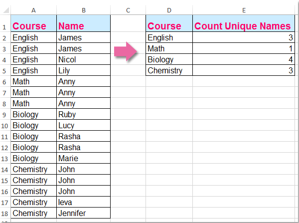
Morda je običajno, da unikatne vrednosti štejemo samo v enem stolpcu, v tem članku pa bom govoril o tem, kako šteti unikatne vrednosti na podlagi drugega stolpca. Na primer, imam naslednja dva stolpca, zdaj moram prešteti unikatna imena v stolpcu B glede na vsebino stolpca A, da dobim naslednji rezultat:

Upoštevajte edinstvene vrednosti na podlagi drugega stolpca z matrično formulo


puščica modri desni mehurček Upoštevajte edinstvene vrednosti na podlagi drugega stolpca z matrično formulo

Če želite odpraviti to težavo, vam lahko pomaga naslednja formula: Naredite naslednje:

1. Vnesite to formulo: =SUMPRODUCT((($A$2:$A$18=D2))/COUNTIFS($A$2:$A$18,$A$2:$A$18&"",$B$2:$B$18,$B$2:$B$18&"")) v prazno celico, kamor želite dati rezultat, E2, na primer. In nato pritisnite Ctrl + Shift + Enter da dobite pravilen rezultat, glejte posnetek zaslona:

doc count edinstven po kriterijih 2

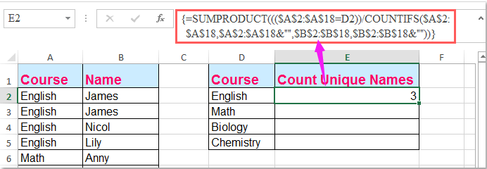
Opombe: V zgornji formuli: A2: A18 so podatki stolpcev, na podlagi katerih štejete unikatne vrednosti, B2: B18 je stolpec, v katerega želite prešteti edinstvene vrednosti, D2 vsebuje merila, na podlagi katerih štejete.

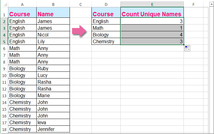
2. Nato povlecite ročico za polnjenje navzdol, da dobite edinstvene vrednosti ustreznih meril. Oglejte si posnetek zaslona:

doc count edinstven po kriterijih 3


Sorodni članki:

Kako prešteti število enoličnih vrednosti v obsegu v Excelu?

Kako prešteti enolične vrednosti v filtriranem stolpcu v Excelu?

Kako šteti enake ali podvojene vrednosti samo enkrat v stolpec?

Najboljša pisarniška orodja za produktivnost

🤖 Kutools AI Aide: Revolucionirajte analizo podatkov na podlagi: Inteligentna izvedba   |  Ustvari kodo  |  Ustvarite formule po meri  |  Analizirajte podatke in ustvarite grafikone  |  Prikličite funkcije Kutools...
Priljubljene funkcije: Poiščite, označite ali identificirajte dvojnike   |  Izbriši prazne vrstice   |  Združite stolpce ali celice brez izgube podatkov   |   Krog brez formule ...
Super iskanje: Več kriterijev VLookup    Multiple Value VLookup  |   VLookup na več listih   |   Nejasno iskanje ....
Napredni spustni seznam: Hitro ustvarite spustni seznam   |  Odvisni spustni seznam   |  Večkrat izberite spustni seznam ....
Upravitelj stolpcev: Dodajte določeno število stolpcev  |  Premakni stolpce  |  Preklop stanja vidnosti skritih stolpcev  |  Primerjaj obsege in stolpce ...
Predstavljene funkcije: Mrežni fokus   |  Pogled oblikovanja   |   Velika vrstica formule    Upravitelj delovnih zvezkov in listov   |  Knjižnica virov (Samodejno besedilo)   |  Izbirnik datuma   |  Združite delovne liste   |  Šifriranje/dešifriranje celic    Pošljite e-pošto po seznamu   |  Super filter   |   Poseben filter (filter krepko/ležeče/prečrtano ...) ...
15 najboljših kompletov orodij12 Besedilo Orodja (dodajanje besedila, Odstrani znake,...)   |   50 + Graf Vrste (Gantt Chart,...)   |   40+ Praktično Formule (Izračunajte starost glede na rojstni dan,...)   |   19 vstavljanje Orodja (Vstavite kodo QR, Vstavi sliko s poti,...)   |   12 Pretvorba Orodja (Številke v besede, Pretvorba valut,...)   |   7 Spoji in razdeli Orodja (Napredne kombinirane vrstice, Razdeljene celice,...)   |   ... in več

Napolnite svoje Excelove spretnosti s Kutools za Excel in izkusite učinkovitost kot še nikoli prej. Kutools za Excel ponuja več kot 300 naprednih funkcij za povečanje produktivnosti in prihranek časa.  Kliknite tukaj, če želite pridobiti funkcijo, ki jo najbolj potrebujete...

Opis


Kartica Office prinaša vmesnik z zavihki v Office in poenostavi vaše delo

  • Omogočite urejanje in branje z zavihki v Wordu, Excelu, PowerPointu, Publisher, Access, Visio in Project.
  • Odprite in ustvarite več dokumentov v novih zavihkih istega okna in ne v novih oknih.
  • Poveča vašo produktivnost za 50%in vsak dan zmanjša na stotine klikov miške za vas!
Comments (20)
No ratings yet. Be the first to rate!
This comment was minimized by the moderator on the site
Hi, thanks for this formula, I'm having an issue implementing it across two Worksheets. In my example, your columns A and B are on one sheet, and D and E are on another, which collects similar data from other year-based Sheets. If I put the formula on the sheet where D (Area) and E are, in E it just returns a zero =SUMPRODUCT(((MHST2324[@Team]=[@Area]))/COUNTIFS(MHST2324[@Team],MHST2324[@Team]&"",MHST2324[@School],MHST2324[@School]&"")). However if I put the formula on the Sheet where A (Team) and B (School) are, it works =SUMPRODUCT((([@Team]=Schools[Area]))/COUNTIFS([@Team],[@Team]&"",[@School],[@School]&"")), any ideas as to why?
This comment was minimized by the moderator on the site
Hey, thanks for this formula, I'm having a problem where
This comment was minimized by the moderator on the site
Классная формула, но как сделать чтобы в столбец A и B можно было постоянно добавлять и не менять формулу ? закрепить не диапазон а столбцы
This comment was minimized by the moderator on the site
Hello, DM,
In fact, you can enlarg the cell references as you need. For example:
=SUMPRODUCT((($A$2:$A$10000=D2))/COUNTIFS($A$2:$A$10000,$A$2:$A$10000&"",$B$2:$B$10000,$B$2:$B$10000&""))
Please remeber to press Ctrl + Shift + Enter keys together.
Please have a try, hope it can help you!
This comment was minimized by the moderator on the site
Is there a way to do this but not count a blank cell as a value?
This comment was minimized by the moderator on the site
Hello, MB
To count the unqiue values with criteria and skip the blank cell, you should apply the below array formula:
=SUM(--(FREQUENCY(IF($B$2:$B$15<>"",IF($A$2:$A$15=D2,MATCH($B$2:$B$15,$B$2:$B$15,0))),ROW($B$2:$B$15)-ROW(B2)+1)>0))


After pasting the fromula, please press Ctrl + Shift + Enter keys together.

https://www.extendoffice.com/images/stories/comments/comment-skyyang/doc-count-unique-criteria.png

Please try, hope it can help you!
This comment was minimized by the moderator on the site
Thank you very much for this but how does it work with a large data set. I realised it returns #N/A when the data is beyond row 78
This comment was minimized by the moderator on the site
I would need to do something similar but with dates: on a sheet in which the dates are indicated in the first column, many repeated, I would like to know how many different dates there are that meet a certain condition that appears in another column. I am applying that formula but it gives me an error. Could you help me? Thanks.
This comment was minimized by the moderator on the site
Does anyone know what the ampersand-quotes (" &"" ") in the Criteria 1 and 2 portion of the COUNTIFS formula is doing? This formula worked for me I was just hoping to understand it better.
This comment was minimized by the moderator on the site
Worked like a charm. Very much greatful to you.
This comment was minimized by the moderator on the site
OMG.... I have been searching for over a week for a formula that came close to helping me do a distinct count of one column based on another column.... YOURS FINALLY HELPED ;0) I am so happy!!!!!! Now I just need this formula that you posted to do the same thing but based on 2 column instead of one. I am going to try on my own but do you think you can help?
This comment was minimized by the moderator on the site
Hello, EB, To count the unique values based on two columns, please apply the below formula, after entering the formula, please press Ctrl + Shift + Enter keys together to get the correct result.=SUM(IFERROR(($A$2:$A$15=E2)*($B$2:$B$15=F2)/COUNTIFS($C$2:$C$15,$C$2:$C$15,$A$2:$A$15,E2,$B$2:$B$15,F2),0))
Please try, hope it can help you!
This comment was minimized by the moderator on the site
WOAH, you're a savior, thank you for sharing
This comment was minimized by the moderator on the site
Nevermind it did
There are no comments posted here yet
Load More
Please leave your comments in English
Posting as Guest
×
Rate this post:
0   Characters
Suggested Locations