Kako vlookup številke, shranjene kot besedilo v Excelu?

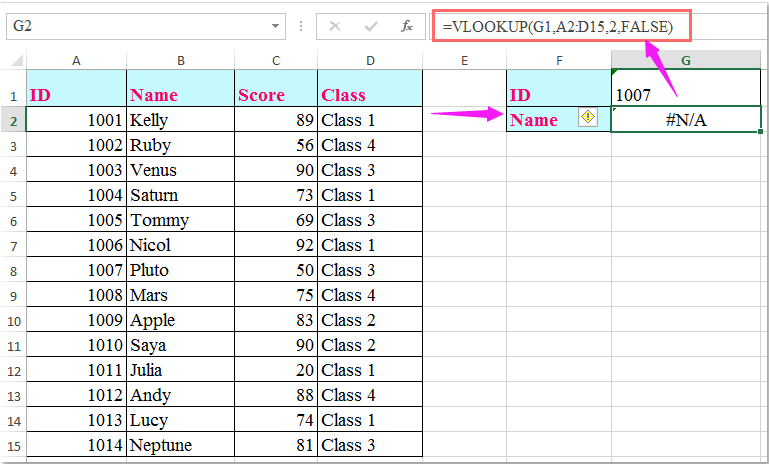
Recimo, da imam naslednji obseg podatkov, ID številka v izvirni tabeli je format številke, v iskalni celici, ki je shranjena kot besedilo, ko uporabim normalno funkcijo VLOOKUP, bom dobil rezultat napake, kot je prikazano spodaj na sliki zaslona. V tem primeru, kako naj dobim pravilne podatke, če imata izbirna številka in izvirna številka v tabeli različno obliko zapisa podatkov?

Vlookup številke, shranjene kot besedilo s formulami

Vlookup številke, shranjene kot besedilo s formulami

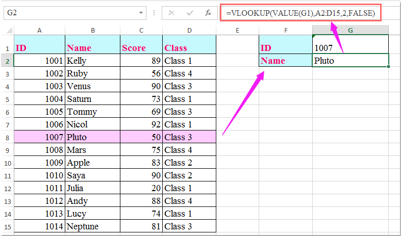
Če je vaša iskalna številka shranjena kot besedilo in je izvirna številka v tabeli v obliki resnične številke, uporabite naslednjo formulo, da vrnete pravilen rezultat:

Vnesite to formulo: = OGLED (VREDNOST (G1), A2: D15,2, FALSE) v prazno celico, kjer želite poiskati rezultat, in pritisnite Vnesite tipko za vrnitev ustreznih podatkov, ki jih potrebujete, glejte posnetek zaslona:

Opombe:

1. V zgornji formuli: G1 je merilo, ki ga želite iskati, A2: D15 je obseg tabel, ki vsebuje podatke, ki jih želite uporabiti, in številko 2 označuje številko stolpca, ki ima ustrezno vrednost, ki jo želite vrniti.

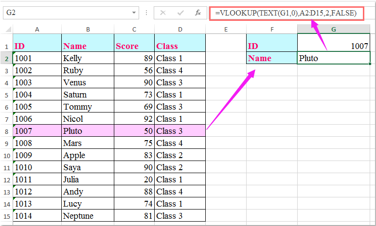
2. Če je vaša iskalna vrednost v obliki številke in je številka ID v izvirni tabeli shranjena kot besedilo, zgornja formula ne bo delovala, uporabite to formulo: = PREGLED (BESEDILO (G1,0), A2: D15,2, FALSE) da dobite pravi rezultat, kot ga potrebujete.

3. Če niste prepričani, kdaj boste imeli številke in kdaj besedilo, lahko uporabite to formulo: =IFERROR(VLOOKUP(VALUE(G1),A2:D15,2,0),VLOOKUP(TEXT(G1,0),A2:D15,2,0)) obravnavati oba primera.

Najboljša pisarniška orodja za produktivnost

🤖	Kutools AI Aide: Revolucionirajte analizo podatkov na podlagi: Inteligentna izvedba   |  Ustvari kodo  |  Ustvarite formule po meri  |  Analizirajte podatke in ustvarite grafikone  |  Prikličite funkcije Kutools...
	Priljubljene funkcije: Poiščite, označite ali identificirajte dvojnike   |  Izbriši prazne vrstice   |  Združite stolpce ali celice brez izgube podatkov   |   Krog brez formule ...
	Super iskanje: Več kriterijev VLookup  |   Multiple Value VLookup  |   VLookup na več listih   |   Nejasno iskanje ....
	Napredni spustni seznam: Hitro ustvarite spustni seznam   |  Odvisni spustni seznam   |  Večkrat izberite spustni seznam ....
	Upravitelj stolpcev: Dodajte določeno število stolpcev  |  Premakni stolpce  |  Preklop stanja vidnosti skritih stolpcev  |  Primerjaj obsege in stolpce ...
	Predstavljene funkcije: Mrežni fokus   |  Pogled oblikovanja   |   Velika vrstica formule   |  Upravitelj delovnih zvezkov in listov   |  Knjižnica virov (Samodejno besedilo)   |  Izbirnik datuma   |  Združite delovne liste   |  Šifriranje/dešifriranje celic   |  Pošljite e-pošto po seznamu   |  Super filter   |   Poseben filter (filter krepko/ležeče/prečrtano ...) ...
	15 najboljših kompletov orodij:  12 Besedilo Orodja (dodajanje besedila, Odstrani znake,...)   |   50 + Graf Vrste (Gantt Chart,...)   |   40+ Praktično Formule (Izračunajte starost glede na rojstni dan,...)   |   19 vstavljanje Orodja (Vstavite kodo QR, Vstavi sliko s poti,...)   |   12 Pretvorba Orodja (Številke v besede, Pretvorba valut,...)   |   7 Spoji in razdeli Orodja (Napredne kombinirane vrstice, Razdeljene celice,...)   |   ... in več

Napolnite svoje Excelove spretnosti s Kutools za Excel in izkusite učinkovitost kot še nikoli prej. Kutools za Excel ponuja več kot 300 naprednih funkcij za povečanje produktivnosti in prihranek časa.  Kliknite tukaj, če želite pridobiti funkcijo, ki jo najbolj potrebujete...

Preberite več ... Brezplačen prenos...

---

Kartica Office prinaša vmesnik z zavihki v Office in poenostavi vaše delo

• Omogočite urejanje in branje z zavihki v Wordu, Excelu, PowerPointu, Publisher, Access, Visio in Project.
• Odprite in ustvarite več dokumentov v novih zavihkih istega okna in ne v novih oknih.
• Poveča vašo produktivnost za 50%in vsak dan zmanjša na stotine klikov miške za vas!

Preberite več ... Brezplačen prenos...