Preskoči na glavno vsebino

Kako prešteti število pojavitev v stolpcu na Googlovem listu?

Avtor: Xiaoyang Zadnja sprememba: 2020-04-23

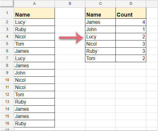
Recimo, da imate seznam imen v stolpcu A Googlovega lista, zdaj pa želite prešteti, kolikokrat se posamezno ime prikaže, kot je prikazano na spodnji sliki zaslona. V tej vadnici bom govoril o nekaterih formulah za reševanje tega dela v Googlovem listu.

Štejte število pojavitev v stolpcu na Googlovem listu s pomožno formulo

Štejte število pojavitev v stolpcu na Googlovem listu s formulo


Štejte število pojavitev v stolpcu na Googlovem listu s pomožno formulo

Pri tej metodi lahko najprej iz stolpca izvlečete vsa unikatna imena in nato štetje pojavnosti na podlagi unikatne vrednosti.

1. Vnesite to formulo: = ENOTNA (A2: A16) v prazno celico, kjer želite izvleči edinstvena imena, in pritisnite Vnesite ključ, vse edinstvene vrednosti so bile navedene na spodnji sliki:

Opombe: V zgornji formuli, A2: A16 so podatki stolpca, ki jih želite šteti.

2. In nato nadaljujte s to formulo: = ŠTEVILO (A2: A16, C2) poleg prve celice formule pritisnite Vnesite tipko, da dobite prvi rezultat, in nato povlecite ročico za polnjenje navzdol do celic, v katere želite prešteti pojavnost edinstvenih vrednosti, glejte posnetek zaslona:

Opombe: V zgornji formuli, A2: A16 so podatki stolpcev, od katerih želite šteti unikatna imena, in C2 je prva edinstvena vrednost, ki ste jo izvlekli.


Štejte število pojavitev v stolpcu na Googlovem listu s formulo

Za rezultat lahko uporabite tudi naslednjo formulo. Naredite to:

Vnesite to formulo: = ArrayFormula (QUERY (A1: A16 & {"", ""}, "izberite Col1, count (Col2) where Col1! = '' Group by Col1 label count (Col2) 'Count'", 1)) v prazno celico, kamor želite postaviti rezultat, nato pritisnite Vnesite in izračunani rezultat se prikaže naenkrat, glejte posnetek zaslona:

Opombe: V zgornji formuli, A1: A16 je obseg podatkov, ki vključuje glavo stolpca, ki jo želite šteti.


Štetje števila pojavitev v stolpcu v programu Microsoft Excel:

Kutools za ExcelJe Napredne kombinirane vrstice pripomoček vam lahko pomaga prešteti število pojavitev v stolpcu, prav tako pa vam lahko pomaga združiti ali sešteti ustrezne vrednosti celic na podlagi istih celic v drugem stolpcu.

Kutools za Excel: z več kot 300 priročnimi dodatki za Excel, brezplačno preizkusite brez omejitev v 30 dneh. Prenesite in brezplačno preskusite zdaj!

Najboljša pisarniška orodja za produktivnost

🤖 Kutools AI Aide: Revolucionirajte analizo podatkov na podlagi: Inteligentna izvedba   |  Ustvari kodo  |  Ustvarite formule po meri  |  Analizirajte podatke in ustvarite grafikone  |  Prikličite funkcije Kutools...
Priljubljene funkcije: Poiščite, označite ali identificirajte dvojnike   |  Izbriši prazne vrstice   |  Združite stolpce ali celice brez izgube podatkov   |   Krog brez formule ...
Super iskanje: Več kriterijev VLookup    Multiple Value VLookup  |   VLookup na več listih   |   Nejasno iskanje ....
Napredni spustni seznam: Hitro ustvarite spustni seznam   |  Odvisni spustni seznam   |  Večkrat izberite spustni seznam ....
Upravitelj stolpcev: Dodajte določeno število stolpcev  |  Premakni stolpce  |  Preklop stanja vidnosti skritih stolpcev  |  Primerjaj obsege in stolpce ...
Predstavljene funkcije: Mrežni fokus   |  Pogled oblikovanja   |   Velika vrstica formule    Upravitelj delovnih zvezkov in listov   |  Knjižnica virov (Samodejno besedilo)   |  Izbirnik datuma   |  Združite delovne liste   |  Šifriranje/dešifriranje celic    Pošljite e-pošto po seznamu   |  Super filter   |   Poseben filter (filter krepko/ležeče/prečrtano ...) ...
15 najboljših kompletov orodij12 Besedilo Orodja (dodajanje besedila, Odstrani znake,...)   |   50 + Graf Vrste (Gantt Chart,...)   |   40+ Praktično Formule (Izračunajte starost glede na rojstni dan,...)   |   19 vstavljanje Orodja (Vstavite kodo QR, Vstavi sliko s poti,...)   |   12 Pretvorba Orodja (Številke v besede, Pretvorba valut,...)   |   7 Spoji in razdeli Orodja (Napredne kombinirane vrstice, Razdeljene celice,...)   |   ... in več

Napolnite svoje Excelove spretnosti s Kutools za Excel in izkusite učinkovitost kot še nikoli prej. Kutools za Excel ponuja več kot 300 naprednih funkcij za povečanje produktivnosti in prihranek časa.  Kliknite tukaj, če želite pridobiti funkcijo, ki jo najbolj potrebujete...

Opis


Kartica Office prinaša vmesnik z zavihki v Office in poenostavi vaše delo

  • Omogočite urejanje in branje z zavihki v Wordu, Excelu, PowerPointu, Publisher, Access, Visio in Project.
  • Odprite in ustvarite več dokumentov v novih zavihkih istega okna in ne v novih oknih.
  • Poveča vašo produktivnost za 50%in vsak dan zmanjša na stotine klikov miške za vas!
Comments (14)
No ratings yet. Be the first to rate!
This comment was minimized by the moderator on the site
可以限制规定内容出现的频次吗
This comment was minimized by the moderator on the site
Thanks!!! how do I count multiple columns?Ie column A, B,C,D all have names that needs to be counted
This comment was minimized by the moderator on the site
Thank you for this! Been trying to figure it out for hours!
This comment was minimized by the moderator on the site
Hi, I am trying to filter out some data from a sheet that is regularly updated. To simplify keeping track of the data I have a reporting section on the google sheet.The problem is that the data isn't organized in the most ideal way.

There are 2 columns that I want to use specific data from to create a filter, then with the leftover names I want to know how many unique names there are


Column 1 - Filter with A for one report field, B for the other report field (I will manually change this in the formula)

Column 2 - There are 9 Text entries possible. I want to only include 3 of them as a Filter

Column 3 - There are a couple of thousand entries(names), many are the same in multiple rows. With the data filtered using Column 1, and Column 2, I want to get a number for how many unique names are left after the data has been filtered.


I am not used to having this many things I am trying to filter the data from so any help would be hugely appreciated.


Have an excellent day
This comment was minimized by the moderator on the site
I have a google sheet with a lot of information but I am looking to filter it down into a report.

Column1 - Options are A, B (The is the first data to sort)
Column 2 - has 3 of the text string that I want my sum to include, but I want to leave out the others 5.
Column 3 - Names that I want to know how many unique names there are

What I am looking to figure out is the following

Option A, the sum to only include 3 text string that appears multiple times in a 2nd column, The total being how many unique names there are in Column 3

Hoping someone can help as this is a bit over my experience level
This comment was minimized by the moderator on the site
My count isn't grouping the names together.
i.e.
Column B says
Independence
Walnut St.
Parkway
Walnut St.
and instead of my " count " column saying Walnut St. 2 it says
Walnut St. 1
Walnut St. 1

How can I fix this ?
This comment was minimized by the moderator on the site
This is partly what I'm looking for.
Now my next issue is, how can I sort these so that I get them in desending order?
So it should be looking like this:
James 4
Nicol 3
Ruby 3
Lucy 2
Tom 2
John 1

Hope you can help with that as well
This comment was minimized by the moderator on the site
Hi,
If you want to sort the results in descending order, you just need to sort the data by the formula result column after getting the result.
Hope it can help you!
This comment was minimized by the moderator on the site
Whenever I try to sort, I get an error, is there a way I can fix that? I have the $A$1:$A$7, B1 as my formula - is there something in my formula I should edit?
This comment was minimized by the moderator on the site
VERY useful - thank you so much!
This comment was minimized by the moderator on the site
Thanks! Super useful!
This comment was minimized by the moderator on the site
When you drag the handle down to apply it to the rest of the values, it increments the search radius by 1. So if youre searching =COUNTIF(A1:A10,C1), when you drag the handle down, the second value will be =COUNTIF(A2:A11,C2).
This comment was minimized by the moderator on the site
This is SOOO helpful! This skips an entire step
This comment was minimized by the moderator on the site
You fix it this way
=COUNTIF($A$2:$A$11,C2)
There are no comments posted here yet
Please leave your comments in English
Posting as Guest
×
Rate this post:
0   Characters
Suggested Locations