Preskoči na glavno vsebino

Kako skriti nič podatkovnih nalepk v grafikonu v Excelu?

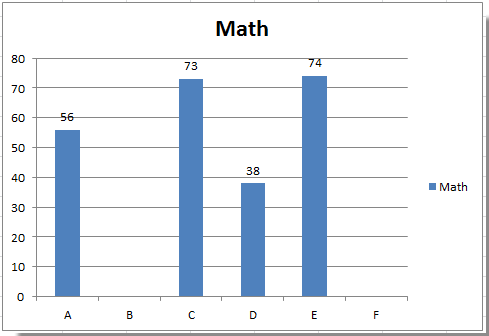
Včasih lahko v grafikon dodate podatkovne nalepke, da v Excelu naredijo vrednost podatkov bolj jasno in neposredno. Toda v nekaterih primerih na grafikonu ni nobenih podatkovnih nalepk, zato boste morda želeli te nič podatkovne nalepke skriti. Tukaj vam bom povedal hiter način, da naenkrat v Excelu skrijete nič podatkovnih nalepk.

V grafikonu skrijete nič podatkovnih nalepk


puščica modri desni mehurček V grafikonu skrijete nič podatkovnih nalepk

Če želite v grafikonu skriti nič podatkovnih nalepk, storite naslednje:

1. Z desno miškino tipko kliknite eno od podatkovnih nalepk in izberite Oblikujte oznake podatkov iz kontekstnega menija. Oglejte si posnetek zaslona:

doc-hide-zero-data-label-1

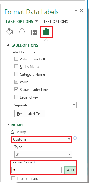
2. V Ljubljani Oblikujte oznake podatkov pogovorno okno, kliknite Število v levem podoknu, nato izberite Po meri iz kategorije polje in vnesite # "" v Koda oblike polje in kliknite Dodaj , če ga želite dodati tip seznamsko polje. Oglejte si posnetek zaslona:

doc-hide-zero-data-label-2

3. klik Zapri , da zaprete pogovorno okno. Potem lahko vidite, da so vse oznake nič podatkov skrite.

doc-hide-zero-data-label-3

Nasvet: Če želite prikazati oznake ničelnih podatkov, se vrnite v pogovorno okno Format Data Labels in kliknite Število > po meriin izberite #, ## 0; - #, ## 0 v tip seznamsko polje.

Opombe: V Excelu 2013 lahko z desno miškino tipko kliknete katero koli podatkovno nalepko in izberete Oblikujte oznake podatkov da odprete Oblikujte oznake podatkov podokno; nato kliknite Število razširiti svojo možnost; nato kliknite Kategorija in izberite polje po meri s spustnega seznama in vnesite # "" v Koda oblike in kliknite Dodaj gumb.

doc-hide-zero-data-label-4


Relativni članki:

Najboljša pisarniška orodja za produktivnost

🤖 Kutools AI Aide: Revolucionirajte analizo podatkov na podlagi: Inteligentna izvedba   |  Ustvari kodo  |  Ustvarite formule po meri  |  Analizirajte podatke in ustvarite grafikone  |  Prikličite funkcije Kutools...
Priljubljene funkcije: Poiščite, označite ali identificirajte dvojnike   |  Izbriši prazne vrstice   |  Združite stolpce ali celice brez izgube podatkov   |   Krog brez formule ...
Super iskanje: Več kriterijev VLookup    Multiple Value VLookup  |   VLookup na več listih   |   Nejasno iskanje ....
Napredni spustni seznam: Hitro ustvarite spustni seznam   |  Odvisni spustni seznam   |  Večkrat izberite spustni seznam ....
Upravitelj stolpcev: Dodajte določeno število stolpcev  |  Premakni stolpce  |  Preklop stanja vidnosti skritih stolpcev  |  Primerjaj obsege in stolpce ...
Predstavljene funkcije: Mrežni fokus   |  Pogled oblikovanja   |   Velika vrstica formule    Upravitelj delovnih zvezkov in listov   |  Knjižnica virov (Samodejno besedilo)   |  Izbirnik datuma   |  Združite delovne liste   |  Šifriranje/dešifriranje celic    Pošljite e-pošto po seznamu   |  Super filter   |   Poseben filter (filter krepko/ležeče/prečrtano ...) ...
15 najboljših kompletov orodij12 Besedilo Orodja (dodajanje besedila, Odstrani znake,...)   |   50 + Graf Vrste (Gantt Chart,...)   |   40+ Praktično Formule (Izračunajte starost glede na rojstni dan,...)   |   19 vstavljanje Orodja (Vstavite kodo QR, Vstavi sliko s poti,...)   |   12 Pretvorba Orodja (Številke v besede, Pretvorba valut,...)   |   7 Spoji in razdeli Orodja (Napredne kombinirane vrstice, Razdeljene celice,...)   |   ... in več

Napolnite svoje Excelove spretnosti s Kutools za Excel in izkusite učinkovitost kot še nikoli prej. Kutools za Excel ponuja več kot 300 naprednih funkcij za povečanje produktivnosti in prihranek časa.  Kliknite tukaj, če želite pridobiti funkcijo, ki jo najbolj potrebujete...

Opis


Kartica Office prinaša vmesnik z zavihki v Office in poenostavi vaše delo

  • Omogočite urejanje in branje z zavihki v Wordu, Excelu, PowerPointu, Publisher, Access, Visio in Project.
  • Odprite in ustvarite več dokumentov v novih zavihkih istega okna in ne v novih oknih.
  • Poveča vašo produktivnost za 50%in vsak dan zmanjša na stotine klikov miške za vas!
Comments (15)
No ratings yet. Be the first to rate!
This comment was minimized by the moderator on the site
Muito obrigado!
This comment was minimized by the moderator on the site
Depending on your data set, you could use a helper column. The formula could use rounddown or IF(cell<1,0,cell). This way your slicers stay intact and your pie chart uses the new column.
This comment was minimized by the moderator on the site
I have a pivot chart (pie chart) where I need to remove the labels for any slice of the pie with a value under 1%. Right now, these are displayed as 0% (no decimal places). I am also using slicers to analyse the data by month, department and person. I am trying to get the chart to hide any labels where the value is less than 1%, but this will change when I change the variables in the slicers. I have fallen down a rabbit-hole here trying to figure this out.
This comment was minimized by the moderator on the site
The Microsoft way of doing it (though not found on ana MS help page) is to click File>Options>Advanced, scroll down to 'Display options for this worksheet', and uncheck / untick 'Show a zero in cells that have a zero value'. All the zeros disappear.

I seem to have found a way to remove the axis name and space on a graph or chart for zero values: Highlight the whole table, click Home>Sort and filter>Filter, Click on the header of the column with the blank zero values, and uncheck / untick 'Blanks'.
This comment was minimized by the moderator on the site
Thanks that really works well for me.
This comment was minimized by the moderator on the site
tnx, it works
This comment was minimized by the moderator on the site
How can I hide Zero Data Labels when it is percentage (for example 0,00%, I do not want that label to be shown)?
This comment was minimized by the moderator on the site
<span style="letter-spacing: 0.2px; color: inherit; font-family: inherit; font-style: inherit; font-variant-ligatures: inherit; font-variant-caps: inherit; font-weight: inherit;">0.0%;-0.0%;""    </span>
This comment was minimized by the moderator on the site
Hi
Thank you for sharing the solution above. It was really great help. However, after hiding zero values, I am having difficulties with hiding their labels. Can you please give a solution for that problem, too? Thank in advance for your help.
This comment was minimized by the moderator on the site
Found this solution absolutely useful. Thanks a ton.
This comment was minimized by the moderator on the site
Great solution! Can this be done retaining decimal points on the numbers that do appear?
This comment was minimized by the moderator on the site
Kelcey, use: #,##"";-#,##""; When using the second semicolon, you define what happens in case of zero. So, if you don't define anything, the value stays blank.
This comment was minimized by the moderator on the site
I use 0.0;;; and it also does the trick, in terms of retaining decimal places. You'd just adjust to the # of sig figs you want to keep. You have to assign the custom value to each data label series, but it keeps that format each time you refresh the data.
There are no comments posted here yet
Load More
Please leave your comments in English
Posting as Guest
×
Rate this post:
0   Characters
Suggested Locations