Preskoči na glavno vsebino

Kako združiti celice, če enaka vrednost obstaja v drugem stolpcu v Excelu?

Kot je prikazano na spodnjem posnetku zaslona, ​​če želite združiti celice v drugem stolpcu na podlagi istih vrednosti v prvem stolpcu, lahko uporabite več metod. V tem članku bomo predstavili tri načine za izpolnitev te naloge.

kombiniraj, če enako


Združi celice, če je enaka vrednost s formulami in filtrom

Naslednje formule pomagajo združiti vsebino ustreznih celic v stolpcu na podlagi iste vrednosti v drugem stolpcu.

1. Izberite prazno celico poleg drugega stolpca (tukaj izberemo celico C2), vnesite formulo = IF (A2 <> A1, B2, C1 & "," & B2) v vrstico s formulami in pritisnite tipko Vnesite ključ.

2. Nato izberite celico C2 in povlecite ročico za polnjenje navzdol do celic, ki jih želite združiti.

3. Vnesite formulo = IF (A2 <> A3, CONCATENATE (A2, "," "", C2, "" ""), "") v celico D2 in povlecite Ročico za polnjenje navzdol do preostalih celic.

4. Izberite celico D1 in kliknite datum > filter. Oglejte si posnetek zaslona:

5. Kliknite puščico spustnega menija v celici D1, počistite polje (Prazne) in nato kliknite OK gumb.

Ogledate si lahko, da so celice združene, če so vrednosti prvega stolpca enake.

Opombe: Za uspešno uporabo zgornjih formul morajo biti enake vrednosti v stolpcu A neprekinjene.


Preprosto združite celice, če je enaka vrednost, s Kutools za Excel (več klikov)

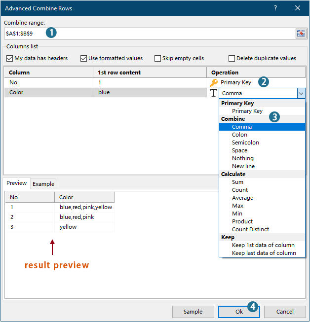
Zgoraj opisana metoda zahteva ustvarjanje dveh pomožnih stolpcev in vključuje več korakov, kar je lahko neprijetno. Če iščete enostavnejši način, razmislite o uporabi Napredne kombinirane vrstice orodje iz Kutools za Excel. S samo nekaj kliki vam ta pripomoček omogoča združevanje celic z uporabo določenega ločila, zaradi česar je postopek hiter in brez težav.

Nasvet: Preden uporabite to orodje, namestite Kutools za Excel najprej. Pojdite na brezplačen prenos zdaj.

1. klik Kutools > Spoji in razdeli > Napredne kombinirane vrstice da omogočite to funkcijo.
2. V Ljubljani Napredne kombinirane vrstice pogovorno okno, morate samo:
  • Izberite obseg, ki ga želite združiti;
  • Nastavite stolpec z enakimi vrednostmi kot Primarni ključ stolpec.
  • Določite ločilo za združevanje celic.
  • klik OK.

Rezultat

Opombe:

Združi celice, če ima enako vrednost s kodo VBA

Kodo VBA lahko uporabite tudi za združevanje celic v stolpcu, če ista vrednost obstaja v drugem stolpcu.

1. Pritisnite druga + F11 tipke za odpiranje Aplikacije Microsoft Visual Basic okno.

2. V Ljubljani Aplikacije Microsoft Visual Basic okno, kliknite Vstavi > Moduli. Nato kopirajte in prilepite spodnjo kodo v Moduli okno.

Koda VBA: združite celice, če imajo enake vrednosti

Sub ConcatenateCellsIfSameValues()
	Dim xCol As New Collection
	Dim xSrc As Variant
	Dim xRes() As Variant
	Dim I As Long
	Dim J As Long
	Dim xRg As Range
	xSrc    = Range("A1", Cells(Rows.Count, "A").End(xlUp)).Resize(, 2)
	Set xRg = Range("D1")
	On Error Resume Next
	For I = 2 To UBound(xSrc)
		xCol.Add xSrc(I, 1), TypeName(xSrc(I, 1)) & CStr(xSrc(I, 1))
	Next I
	On Error GoTo 0
	ReDim xRes(1 To xCol.Count + 1, 1 To 2)
	xRes(1, 1) = "No"
	xRes(1, 2) = "Combined Color"
	For I = 1 To xCol.Count
		xRes(I + 1, 1) = xCol(I)
		For J = 2 To UBound(xSrc)
			If xSrc(J, 1) = xRes(I + 1, 1) Then
				xRes(I + 1, 2) = xRes(I + 1, 2) & ", " & xSrc(J, 2)
			End If
		Next J
		xRes(I + 1, 2) = Mid(xRes(I + 1, 2), 2)
	Next I
	Set xRg = xRg.Resize(UBound(xRes, 1), UBound(xRes, 2))
	xRg.NumberFormat = "@"
	xRg = xRes
	xRg.EntireColumn.AutoFit
End Sub

Opombe:

1. D1 v skladu Nastavi xRg = obseg ("D1") pomeni, da se bo rezultat začel s celico D1.
2. "Ne"in "Kombinirana barva" v skladu xRes (1, 1) = "Ne" in xRes (1, 2) = "Kombinirana barva" so glave izbranih stolpcev. 

3. Pritisnite F5 tipko za zagon kode, potem boste dobili združene rezultate v določenem obsegu.


Preprosto združite celice, če je enaka vrednost, s Kutools za Excel

Najboljša pisarniška orodja za produktivnost

🤖 Kutools AI Aide: Revolucionirajte analizo podatkov na podlagi: Inteligentna izvedba   |  Ustvari kodo  |  Ustvarite formule po meri  |  Analizirajte podatke in ustvarite grafikone  |  Prikličite funkcije Kutools...
Priljubljene funkcije: Poiščite, označite ali identificirajte dvojnike   |  Izbriši prazne vrstice   |  Združite stolpce ali celice brez izgube podatkov   |   Krog brez formule ...
Super iskanje: Več kriterijev VLookup    Multiple Value VLookup  |   VLookup na več listih   |   Nejasno iskanje ....
Napredni spustni seznam: Hitro ustvarite spustni seznam   |  Odvisni spustni seznam   |  Večkrat izberite spustni seznam ....
Upravitelj stolpcev: Dodajte določeno število stolpcev  |  Premakni stolpce  |  Preklop stanja vidnosti skritih stolpcev  |  Primerjaj obsege in stolpce ...
Predstavljene funkcije: Mrežni fokus   |  Pogled oblikovanja   |   Velika vrstica formule    Upravitelj delovnih zvezkov in listov   |  Knjižnica virov (Samodejno besedilo)   |  Izbirnik datuma   |  Združite delovne liste   |  Šifriranje/dešifriranje celic    Pošljite e-pošto po seznamu   |  Super filter   |   Poseben filter (filter krepko/ležeče/prečrtano ...) ...
15 najboljših kompletov orodij12 Besedilo Orodja (dodajanje besedila, Odstrani znake,...)   |   50 + Graf Vrste (Gantt Chart,...)   |   40+ Praktično Formule (Izračunajte starost glede na rojstni dan,...)   |   19 vstavljanje Orodja (Vstavite kodo QR, Vstavi sliko s poti,...)   |   12 Pretvorba Orodja (Številke v besede, Pretvorba valut,...)   |   7 Spoji in razdeli Orodja (Napredne kombinirane vrstice, Razdeljene celice,...)   |   ... in več

Napolnite svoje Excelove spretnosti s Kutools za Excel in izkusite učinkovitost kot še nikoli prej. Kutools za Excel ponuja več kot 300 naprednih funkcij za povečanje produktivnosti in prihranek časa.  Kliknite tukaj, če želite pridobiti funkcijo, ki jo najbolj potrebujete...

Opis


Kartica Office prinaša vmesnik z zavihki v Office in poenostavi vaše delo

  • Omogočite urejanje in branje z zavihki v Wordu, Excelu, PowerPointu, Publisher, Access, Visio in Project.
  • Odprite in ustvarite več dokumentov v novih zavihkih istega okna in ne v novih oknih.
  • Poveča vašo produktivnost za 50%in vsak dan zmanjša na stotine klikov miške za vas!
Comments (23)
No ratings yet. Be the first to rate!
This comment was minimized by the moderator on the site
thank you very much, the VBA code works very well but I have a question that I can't solve.

NO Color
1 red
1 blue
1 red
1 yellow
2 red
2 yellow


in this case, in column B we have some duplicate colors related to the same number. How can I have an output that only return the values once?

I would like an output like this

NO Color
1 red, blue, yellow
2 red, yellow
This comment was minimized by the moderator on the site
Hi

The second method described in the post can help you solve this problem. After following the steps to specify the settings, checking the Delect Duplicate Values option will delete all duplicates in the combined results.
https://www.extendoffice.com/images/stories/comments/comment-picture-zxm/concatenate.png
This comment was minimized by the moderator on the site
Thank you so much for this formula! It saved hours of investigation! Fantastic work :)
This comment was minimized by the moderator on the site
Hi Crystal,

Thanks for your reply. I'll have to put my thinking hat on again...
Thank you
This comment was minimized by the moderator on the site
Hello, the macro above works great! Thank you. Is it anyway possible (I tried, but not successful) to amend it to concatenate column B (description) based on duplicates in column A (HS code) but also taking column C (origin) in the combination?
So description texts concatenate per HS code per origin.
Also column D(quantity) and column E(value) must be summed per HS code and origin.

A B C D E
HS CODE DESCRIPTION ORIGIN QUANTITY VALUE
5407420000 TWEED CN 10 € 150,00
5407420000 COTTON CN 15 € 250,00
5407420000 POLYESTER TW 5 € 130,00
5407420000 ORGANIC COTTON US 18 € 450,00
5407420000 COTTON US 23 € 780,00
5407420000 VELVET DELUXE CN 20 € 380,00
5407420000 COTTON CN 10 € 120,00
5806310000 TWEED JP 15 € 35,00
5806310000 POLYESTER AU 20 € 78,00
5806310000 TWEED AU 25 € 254,00
5806310000 POLYESTER SG 130 € 888,00
5806310000 COTTON EU 120 € 945,00
5806310000 COTTON FABRIC EU 10 € 80,00


Result shopuld be:

5407420000 TWEED, COTTON, VELVET DULUXE, COTTON, CN 55 € 900,00
5407420000 POLYESTER TW 5 € 130,00
5407420000 ORGANIC COTTON, COTTON US 41 € 1230,00
5806310000 TWEED JP 15 € 35,00
5806310000 POLYESTER, TWEED AU 45 € 332,00
5806310000 POLYESTER SG 130 € 888,00
5806310000 COTTON, COTTON FABRIC EU 130 € 1025,00

I hope this possible, thank you!
This comment was minimized by the moderator on the site
Hi Ivar,

Thank you for your comment. I am not able to solve this problem with VBA code yet. Sorry for that.
You can try if the last method can help.
This comment was minimized by the moderator on the site
Hello, how would the VBA code be adjusted if I want to combine cells in column M based on the duplicates in column A?
This comment was minimized by the moderator on the site
Hi Kristin,To combine cells in column M based on the duplicates in column A, try the VBA below.In the code,  O1 is the first cell to output the results; M is the column you will combine based on the duplicates in column A; A1 and A represent the first cell and the column where the duplicates locate; No and Combine color is the header of the columns after concatenating. You can change these variables as needed.<div data-tag="code">Sub ConcatenateCellsIfSameValues()
'Updated by Extendoffice 20211105
Dim xCol As New Collection
Dim xSrc As Variant
Dim xSrcValue As Variant
Dim xRes() As Variant
Dim I As Long
Dim J As Long
Dim xRg As Range
Dim xResultAddress As String
Dim xMergeAddress As String
Dim xUp As Integer

xResultAddress = "O1" 'The cell to output the results
xMergeAddress = "M" 'The column you will combine based on the duplicates in column A

xSrc = Range("A1", Cells(Rows.Count, "A").End(xlUp)).Resize(, 1)
xUp = Range("A1", Cells(Rows.Count, "A").End(xlUp)).Rows.Count
xSrcValue = Range(xMergeAddress & "1:" & xMergeAddress & xUp)

Set xRg = Range(xResultAddress)
On Error Resume Next
For I = 2 To UBound(xSrc)
xCol.Add xSrc(I, 1), TypeName(xSrc(I, 1)) & CStr(xSrc(I, 1))
Next I

On Error GoTo 0
ReDim xRes(1 To xCol.Count + 1, 1 To 2)
xRes(1, 1) = "No"
xRes(1, 2) = "Combined Color"
For I = 1 To xCol.Count
xRes(I + 1, 1) = xCol(I)
For J = 2 To UBound(xSrc)
If xSrc(J, 1) = xRes(I + 1, 1) Then
xRes(I + 1, 2) = xRes(I + 1, 2) & ", " & xSrcValue(J, 1)
End If
Next J
xRes(I + 1, 2) = Mid(xRes(I + 1, 2), 2)
Next I
Set xRg = xRg.Resize(UBound(xRes, 1), UBound(xRes, 2))
xRg.NumberFormat = "@"
xRg = xRes
xRg.EntireColumn.AutoFit
End Sub
This comment was minimized by the moderator on the site
I just wanted to thank you. It wasn't exactly what I wanted but man did it help me figure out what to do.

I have a table where the person's name was in column A, dates in column B and the names of tools they use in the headers of columns C:G . In each column there is a "Y" if they used that tool on that date and blank if they did not. (FYI: the same person can be listed more than once and may have used the same tool more than once) On a separate (summary) page I wanted to list all tools each person used within a date period, only listing each tool they used once, in the same cell. On this page, the person's name was in column A, Types of tools used in column B and the helper columns were in column G:K. Here's what I got:
The first helper column (G2):
=IF(COUNTIFS(Table7[Person's Name],A2,Table7[Screw Driver],"Y",Table7[Date],">="&1/1/20,Table7[Date],"<="&3/31/20),"Screw Driver","")
In the last helper column (K2):
=IF(COUNTIFS(Table7[Person's Name],A2,Table7[Hammer],"Y",Table7[Date],">="&1/1/20,Table7[Date],"<="&3/31/20),IF(J2="","Hammer",J2&"/"&"Hammer"),J2)

In B2 I just entered =K2

Thanks again and I hope this helps someone. EZPD
This comment was minimized by the moderator on the site
Hi, first of all thanks for creating this resource. I have been trying to figure this out for a couple of hours and I'm stuck. I'm using your 'concatenate cells if same value' but my script is looking at column "D" instead of "A. I can't figure out how to get it to use a different column for the data besides the one right next to it. In my cases I want it to look at column "D" to see if the value is the same and if so, it will grab the data from column "H" and put that data from column "H' into a cell in column "J". How do I switch this to use column "H" for the data? Thx


Sub ConcatenateCellsIfSameValues()
Dim xCol As New Collection
Dim xSrc As Variant
Dim xRes() As Variant
Dim I As Long
Dim J As Long
Dim xRg As Range
xSrc = Range("D1", Cells(Rows.Count, "D").End(xlUp)).Resize(, 2)
Set xRg = Range("J1")
On Error Resume Next
For I = 2 To UBound(xSrc)
xCol.Add xSrc(I, 1), TypeName(xSrc(I, 1)) & CStr(xSrc(I, 1))
Next I
On Error GoTo 0
ReDim xRes(1 To xCol.Count + 1, 1 To 2)
xRes(1, 1) = "No"
xRes(1, 2) = "Products"
For I = 1 To xCol.Count
xRes(I + 1, 1) = xCol(I)
For J = 2 To UBound(xSrc)
If xSrc(J, 1) = xRes(I + 1, 1) Then
xRes(I + 1, 2) = xRes(I + 1, 2) & vbCrLf & xSrc(J, 2)
End If
Next J
xRes(I + 1, 2) = Mid(xRes(I + 1, 2), 2)
Next I
Set xRg = xRg.Resize(UBound(xRes, 1), UBound(xRes, 2))
xRg.NumberFormat = "@"
xRg = xRes
xRg.EntireColumn.AutoFit
End Sub
This comment was minimized by the moderator on the site
"I can't figure out how to get it to use a different column for the data besides the one right next to it. In my cases I want it to look at column 'D' to see if the value is the same and if so, it will grab the data from column 'H' and put that data from column 'H' into a cell in column 'J'."

Did you ever figure this out?
This comment was minimized by the moderator on the site
Hi,

looks like 2 of your formulas are wrong :

=IF(A2<>A3,CONCATENATE(A2,",""",C2,""""),""). You need to change "A2" to "D1". As you'll want to add the string to the previous cell.

same goes for this formula :

=IF(A2<>A1,B2,C1 & "," & B2) : Change C1 to D1.


kind regards


Harry
This comment was minimized by the moderator on the site
I use this VBA for lots of my spreadsheets and its great. But the spreadsheets have become very large 50k+ rows and it doesnt seem to be working any more. If I use it on 1000 rows it works fine but large sets of data it cant seem to cope with. No errors just no results. Any help would be appreciated.
This comment was minimized by the moderator on the site
Hi James,
I tested the code as you mentioned, but it still works well in my case even I set the rows to 1000+.
This comment was minimized by the moderator on the site
Using the VBA macro and getting great results, I have tried tweaking it slightly for my needs but cant get it to work so I hope you can help.

Which bit do I change to make it concat a specific column, not the one directly to the right of the xSrc = Range?

Thanks for your great work!
This comment was minimized by the moderator on the site
Or as a better option, if you had 3 columns instead of 2 and found duplicates in column A (like your example) can you concat column B into a cell and column C into a seperate cell? So if you had columns of Number, Colour, Age, could you concat colour and age into different columns upon finding duplicates in Number? Hope that makes sense!
There are no comments posted here yet
Load More
Please leave your comments in English
Posting as Guest
×
Rate this post:
0   Characters
Suggested Locations