Kako skriti samo del vrednosti celice v Excelu?

Recimo, da imate list s splošnimi informacijami o osebju, nekateri pa so zasebni, na primer številke socialnega zavarovanja. Zdaj želite skriti del teh številk socialnega zavarovanja, kot je prikazano spodaj, kako jih lahko hitro rešite?

Številke socialne varnosti delno skrijete s pomočjo Oblikuj celice

Besedilo ali številko delno skrijete s formulami

Številke socialne varnosti delno skrijete s pomočjo Oblikuj celice

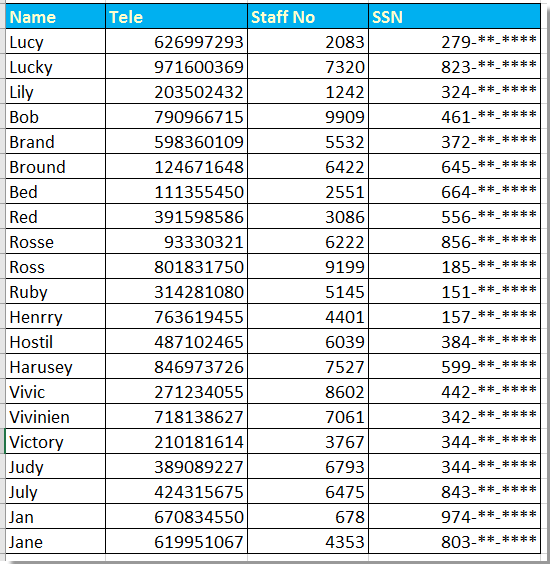
Če želite v Excelu skriti del številk socialne varnosti, lahko za njegovo reševanje uporabite oblikovanje celic.

1. Izberite številke, ki jih želite delno skriti, in z desno miškino tipko izberite Oblikuj celice iz kontekstnega menija. Oglejte si posnetek zaslona:

2. Nato v Oblikuj celice dialog, kliknite Število zavihek in izberite po meri iz Kategorija in pojdite v to 000 ,, "- ** - ****" v tip v desnem delu. Oglejte si posnetek zaslona:

3. klik OK, zdaj so izbrane delne številke skrite.

Opombe： Število bo zaokrožilo, če je četrto število večje od ali eaqul na 5.

Besedilo ali številko delno skrijete s formulami

Z zgornjo metodo lahko skrijete le delne številke, če želite skriti delne številke ali besedila, lahko to storite spodaj:

Tu skrijemo prve 4 številke številke potnega lista.

Izberite eno prazno celico poleg številke potnega lista, na primer F22, vnesite to formulo = "****" & DESNO (E22,5)in nato povlecite ročico za samodejno izpolnjevanje čez celico, ki jo želite uporabiti za to formulo.

Nasvet:

Če želite skriti zadnje štiri številke, uporabite to formulo, = LEVO (H2,5) & "****"

če želite skriti srednje tri številke, uporabite to = LEVO (H2,3) & "***" & DESNO (H2,3)

Najboljša pisarniška orodja za produktivnost

🤖	Kutools AI Aide: Revolucionirajte analizo podatkov na podlagi: Inteligentna izvedba   |  Ustvari kodo  |  Ustvarite formule po meri  |  Analizirajte podatke in ustvarite grafikone  |  Prikličite funkcije Kutools...
	Priljubljene funkcije: Poiščite, označite ali identificirajte dvojnike   |  Izbriši prazne vrstice   |  Združite stolpce ali celice brez izgube podatkov   |   Krog brez formule ...
	Super iskanje: Več kriterijev VLookup  |   Multiple Value VLookup  |   VLookup na več listih   |   Nejasno iskanje ....
	Napredni spustni seznam: Hitro ustvarite spustni seznam   |  Odvisni spustni seznam   |  Večkrat izberite spustni seznam ....
	Upravitelj stolpcev: Dodajte določeno število stolpcev  |  Premakni stolpce  |  Preklop stanja vidnosti skritih stolpcev  |  Primerjaj obsege in stolpce ...
	Predstavljene funkcije: Mrežni fokus   |  Pogled oblikovanja   |   Velika vrstica formule   |  Upravitelj delovnih zvezkov in listov   |  Knjižnica virov (Samodejno besedilo)   |  Izbirnik datuma   |  Združite delovne liste   |  Šifriranje/dešifriranje celic   |  Pošljite e-pošto po seznamu   |  Super filter   |   Poseben filter (filter krepko/ležeče/prečrtano ...) ...
	15 najboljših kompletov orodij:  12 Besedilo Orodja (dodajanje besedila, Odstrani znake,...)   |   50 + Graf Vrste (Gantt Chart,...)   |   40+ Praktično Formule (Izračunajte starost glede na rojstni dan,...)   |   19 vstavljanje Orodja (Vstavite kodo QR, Vstavi sliko s poti,...)   |   12 Pretvorba Orodja (Številke v besede, Pretvorba valut,...)   |   7 Spoji in razdeli Orodja (Napredne kombinirane vrstice, Razdeljene celice,...)   |   ... in več

Napolnite svoje Excelove spretnosti s Kutools za Excel in izkusite učinkovitost kot še nikoli prej. Kutools za Excel ponuja več kot 300 naprednih funkcij za povečanje produktivnosti in prihranek časa.  Kliknite tukaj, če želite pridobiti funkcijo, ki jo najbolj potrebujete...

Preberite več ... Brezplačen prenos...

---

Kartica Office prinaša vmesnik z zavihki v Office in poenostavi vaše delo

• Omogočite urejanje in branje z zavihki v Wordu, Excelu, PowerPointu, Publisher, Access, Visio in Project.
• Odprite in ustvarite več dokumentov v novih zavihkih istega okna in ne v novih oknih.
• Poveča vašo produktivnost za 50%in vsak dan zmanjša na stotine klikov miške za vas!

Preberite več ... Brezplačen prenos...